Anatomy of Latitude Part Two: "Thread with a Needle” in the context of energy

Table of Contents
We continue to explore the magic of energy conversion in a PWM transducer. Why is it magic? Theoretically, as we saw in the previous section, the line stabilizer initially converts some of the useful power into heat, which makes the efficiency of the line stabilizer less than 100%, and it is expected for technical systems. Theoretically, in a PWM transducer this happens without losses, isn't that magic? A PWM transducer, like a tailor with scissors, cuts the “fabric of energy” into pieces, and then, like a sewing machine, stitches the pieces of energy into a dress - DC Magnitude.
What is a constant component and how can we get it? Let's explore!
Pulse Width Modulated Signal - “Pieces of Energy”.
As was said in the previous part, with the keys the energy can be cut in portions in the form of rectangular pulses. They have new properties and characteristics that we must understand in order to apply their properties effectively. Their purpose is to obtain a DC Magnitude of a PWM Signal.
Consider the asymmetrical periodic rectangular signal relative to the horizontal axis:

Where:
- Am - Signal pulse amplitude
- Т - signal period
- tw - pulse duration. When you change it, i.e. the pulse width without T change, the Signal is modulated - that is why the name is Pulse Width Modulation - PWM.
The ratio of the pulse width tw to its period T is called the duty cycle D, and the opposite value is named the off duty ratio S:
D = 1/S = tw/T
In practice, it is more convenient to use the duty cycle for a Signal of the same frequency, which is often expressed as a percentage by multiplying D by 100.
Since the signal is rectangular and asymmetrical, its DC Magnitude is directly affected by D, and therefore it is in strict linear dependence on D and amplitude (Am):
DC Magnitude = Am * D
This important property is used in practice and makes it possible to use the key operating mode of the operating element when applying PWM to our main goal: obtaining a DC Magnitude from a rectangular Signal.
Let's study how PWM works. Create the " PWM Generator work" schematic for this purpose:

V1 is a constant voltage source, that in this case sets D in the range from 0 to 1V (0-100%). We set its value equal to 250mV (i.e. 25%).
U1 is a programmable PWM signal generator (library name: PWM Generator), with an output signal as rectangular pulses with specified frequency. The pulse width is linearly dependent on the input voltage V1 (Vin net), which determines the value of D.
The configurable parameters of the PWM generator are as follows:
- The input (programmable) voltage range Vin must be between MODLOW (corresponds to 0%) and MODHIGH (corresponds to 100%)
- Frequency of the MODFREQ output pulses
- Amplitude of pulses on the Vout output. Minimum value: PWMLOW, Maximum value: PWMHIGH.
The width of the tw pulses is automatically calculated inside the simulator according to the formula:
WIDTH= Vin / ( (MODHIGH - MODLOW ) * MODFREQ )
Configure U1 for convenience:

A DC voltage of 0.25V (D=25%) is applied to input U1 from V1, that according to the formula the pulse width must be 25 ms.
Now let's look at the output. In this case, we need to look at the Signal in the time domain. In the Simulator, we can do this with the following type of analysis: Transient (virtual oscilloscope), which we will configure. We display the signal Vout on a time interval from 0 to 200 ms, with 100 µs step.

Run the Transient calculation (RUN), Look at the chart and make sure that the formula and operation of the circuit model are correct:

When we look at the Signal, we see the DC Magnitude that can be calculated using a calculator, but in this case, it is not complete information about the signal. Because the signal consists not only of one DC Magnitude but also of a number of harmonics, (a number of harmonics of one Signal are the Signal Spectrum).
We must take them into account for practical applications and know their exact composition. In the Simulator there is another great tool that allows you to quickly show the Signal Spectrum - Fourier Analysis. It is located inside the Transient analysis and is activated by ticking the appropriate Fourier Analysis checkbox in the Transient tab:

There are two settings for Fourier Analysis:
- Fundamental Frequency - with this parameter we specify the periodicity of the signal, in our case it is 10Hz;
- Number of Harmonics - how many harmonics we want to see on the spectrum plot.
After configuring Fourier Analysis, run Transient again, and the Fourier Analysis window appears next to the Transient window:

Look, at zero frequency the vertical red line is 250 mV, this is the constant component that we set at the beginning, and to the right, there are the other components of the spectrum. Let's look at the Signal and its spectrum of the opposite case when D=75% (V1=750 mV), the pulse width must be 75 ms and the constant component must be 750 mV:


Compare the spectrum carefully, the constant component has changed from 250 mV to 750 mV, but the other spectral components have not changed at all.
Thus, to solve the energy conversion problem, as we said before, we are interested only in the constant component. Therefore, it is necessary to filter it from ALL non-zero spectral components, and this can be done only with the help of the Low-Pass Filter.
Low-frequency filter - the amazing “sewing machine”
Like a needle in the hands of a tailor, so the filter in the transducer knits the thread out of the fabric of energy...
The low-frequency filter can be realized using two basic methods:
- with RC integrating circuit - this method is widely used where you want to select the constant component as information, and is not suitable for energy conversion, because energy will be dissipated (i.e. simply lost) on R in the form of heat, which is not appropriate for us in this problem.
- with the LC circuit - in this circuit, there is no heat generation and thus no losses, this is the circuit used for energy conversion, and we will now consider it.
Create the following "LPF work" filter schematic in the new project:

For clarity and convenience of further analysis, the schematic is divided into three parts by dotted lines.
The purpose of the Low-frequency filter is to reduce all non-zero harmonics of the spectrum ( alternating components) of the Signal while allocating the DC Magnitude to the load. If we consider the LC circuit separately from the Energy Source, then, given that the internal resistance of the ideal Energy Source is zero, the LC circuit will be a parallel oscillating circuit, with a resonant frequency f0 equal to:
Of course, in order to allocate the constant component, the resonant frequency f0 of this circuit must be lower than the frequency of the first harmonic (otherwise known as the main harmonic) of the PWM signal. When a source of Energy is connected, the LC will become an L-shaped Low-frequency filter with a cut-off frequency of its AFC equal to f0 of the equivalent oscillating circuit.
It is also necessary to consider not the direct characteristic, but the quality Q of the Low-frequency filter and the load as a whole, because when the quality factor is high there may be parasitic emissions at f0 in the load.
In our case the quality factor (Q) is calculated by the following formula:
Q = R1/(√L/C) , where ρ = √L/C is the characteristic impedance of the contour, i.e: Q = R1/ρ
The theory states that depending on the quality factor of the circuit Q, there are four modes of its operation: oscillatory, quasi-oscillatory, critical, and aperiodic:
- Oscillatory, quasi-oscillatory modes are observed at Q>0.5, in these modes resonance phenomena are observed;
- Critical mode at Q=0,5;
- Aperiodic mode at Q<0,5.
For correct suppression of harmonics of PWM signal, Low-frequency filter must work in subcritical mode, i.e. when resonance phenomena do not appear.
Let's study this with the help of the Simulator, but the Simulator must calculate the values of L and C by itself, based on the requirements of the load resistance R1, the frequency of the PWM signal f0, and the total quality factor Q.
After analysis and transformations we get the following:
- The cut-off frequency of the Low frequency filter ftr is (preliminarily) 2 times less than f0: ftr = f0 / 2;
- ρ = R1/Q, and since the resonance frequency of the circuit or cutoff Low frequency filter ρ = XL =XC, then:
- Lf = XL/ (2*Pi*ftr) = ρ/ (2*Pi*ftr);
- Cf = 1/(XC * 2*Pi*ftr) = 1/(ρ * 2*Pi*ftr).
In our task, there are new variables that do not show the equivalent component values on the schematic, but directly ( with formulas) affect them.The Simulator has an excellent tool for applying them (new variables and formulas based on them): Text Frame is a text area where the Simulator takes information for additional description of the Schematic and simulation in the form of global parameters and dependencies based on them.
In our case f0, Q, ftr, Ro, Lf, Cf and the R1 - Rload value are the global parameters, while ftr, Ro, Lf, and Cf are also the result of calculating formulas which include the global parameters: f0, Q, Rload.
To specify the global variables it is necessary to add the Text Frame area in any convenient place of the schematic in Place " Text Frame main menu or by clicking on the icon in the drop-down list in the toolbar. Then you must specify the following:
(Note: * The "+" sign in SPICE is a sign of continuation of the previous line. It is not allowed to use any other symbols before the "+" sign, including space.)
After creating and filling the Text Frame, we assign the values of the global parameters Lf, Cf to L1, C1 according to the schematic, and in the properties of V1 we assign AC Magnitude a value equal to 1 (AC Magnitude is the parameter necessary to start the AC Sweep calculation):

and see the AFC of the Low-frequency filter on the plot without knowing their specific values. In order to do this we need to configure and apply the following type of calculation (AC Sweep).
Knowing that f0=10 Hz, it is necessary to check the AFC of Low-frequency filter at Vload point at least 10 fold scale from this frequency in both directions, i.e. from 1 Hz to 100 Hz, while calculating 100 points per decade of frequency (i.e. the range of frequency change by 10 times):

Run the calculation (RUN) AC Sweep and check the plot:

Note: The frequency scale of the plot is shown on a logarithmic scale. Let's express the amplitude scale also in the logarithmic scale. In order to do this, select the Magnitude (dB) function in +Add Output Expression:

Note that in the Output Expression the Vload function has been updated with the new dB(Vload) function, which logarithms our plot. Press (RUN) AC Sweep again and watch:

The plot reflects the asymptote of the right slope part of the plot. But what is on the left side? We need to see everything there as well. To do this, we just slightly reconfigure the start frequency of the AC Sweep from 1 Hz to 0.01 Hz (i.e. 10 mHz):

If you know the initial data, you can test whether the observed data are correct. To do this, mentally draw two intersecting asymptotes on the chart (in the figure below: two green lines along the straight sections of the chart). The point of intersection will be at 5 Hz, which is the filter cut-off frequency.
ftr = f0 / 2 = 10 / 2 = 5 Hz, which corresponds to the initial data, and hence our considerations and preliminary calculations are correct.

Looking at this chart we can make another interesting conclusion/verification. Any circuit with n reactive components (i.e., an n-order circuit) can give the maximum (non-resonant) slope of the frequency response: n * 20 dB/decade. In our case, Low-frequency filter of 2nd order that has the slope of the right part of the AFC, according to the tangent of the plot, is equal to: (-10 dB (10 Hz) - (-50 dB (100 Hz): (-10 dB (at 10 Hz) - (-50 dB (at 100 Hz)) = 40 dB/decade, which correlates well with the proposed formula.
And what happens if we increase the quality factor Q? For this purpose it is enough to edit line +Q = 0.5 in Text Frame, change Q by 10 times: +Q = 5 and run the calculation:

Let's compare the chart with the previous one:
The purpose of the Low-frequency filter is to suppress all harmonics since the main one (f=10 Hz). At Q=0.5 the fundamental harmonic was attenuated about 14 dB, while at Q=5 the attenuation decreased to 10 dB, i.e. the characteristics of the Low-frequency filter have deteriorated.
When the cutoff frequency was ftr = 5Hz, a highly undesirable strong resonance appeared. It can cause unexpected Feedback in the schematic, which can change the operating modes of the whole schematic.
The slope of the right resonant part of the AFC remained the same -40 dB/decade.
We have seen the effect of the Quality factor of the Low-frequency filter + Load system is critical and oscillatory modes on the characteristics of the Low-frequency filter. And we can draw the main conclusion about its application in our case. When designing a Low-frequency filter to isolate the constant component in the PWM signal, it is necessary that the cut-off frequency must be lower than the main harmonic of the Signal, and pseudo oscillatory and oscillatory modes of operation must be excluded.
Now it's time to see how it all works together, like a sewing shop, where energy like "fabric" is cut with scissors - keys and immediately sewn together with a sewing machine - the low-frequency filter in part three of our story: "The High-Quality Energy Factory"
Related Resources


Related Technical Documentation


Take advantage of the world's
most trusted PCB design system.
One interface. One data
model. Endless possibilities.
Effortlessly collaborate with
mechanical designers.
The world's most trusted
PCB design platform
Best in class interactive
routing
View License Options
Thank you, you are now subscribed to updates.