The Basics of Monte Carlo in SPICE: Theory and Demo

Table of Contents
Anytime you place a component in your PCB, it’s almost like you’re gambling. All components have tolerances, and some of these are very precise (resistors for instance), but others components can have very wide tolerances on their nominal values (e.g., wirewound inductors or ferrites). In the event the tolerances on these components become too large, how can you predict how these tolerances will affect your circuits?
While you could calculate variations around nominal electrical values (voltage, current, or power) by hand, running these calculations by hand is very time consuming, especially in large circuits. However, SPICE simulators have borrowed a very useful type of simulation from probability theory to help you answer these questions. This type of simulation is known as Monte Carlo, and you can now perform this simulation with the SPICE package in Altium Designer.
In this article, I’ll provide an overview of the theory involved in understanding and building Monte Carlo simulations, then I’ll show some example results for a power regulator circuit and how the results are affected by tolerances. Monte Carlo simulations generate a lot of data that you can use to take statistics for your circuit’s operation, and this gives you a good idea of whether your product is highly likely to perform to your specifications due to tolerances on component values.
Monte Carlo in SPICE Simulations
Monte Carlo simulations operate on a simple process: randomly generate a set of numbers, and then use those random numbers in a mathematical model to calculate something useful. When a Monte Carlo simulation is used in SPICE, the simulation generates the component values in your circuit randomly using tolerances that you define. It then uses these randomly generated component values to run a standard SPICE simulation. This process is repeated multiple times (sometimes 100’s of times) to give you a set of data describing how your circuit behavior changes due to component tolerances.
SPICE packages implement Monte Carlo simulations through a simple process. This involves random number generation and calculation of voltage and current in the standard SPICE algorithm, followed by displaying results in a table or graph:
- Select which components you want to experience random variations, and define the tolerance on the component.
- Select a distribution for component tolerances (Gaussian is most commonly used) and the number of simulation runs.
- The SPICE simulator generates random component values using the nominal defined in the schematic and the tolerance/distribution defined in Step 2.
- The SPICE simulator calculates the target voltage/current/power at each point in the circuit using the random component values in Step 3.
- Steps 3 and 4 are repeated until the desired number of simulation runs is reached.
- The results from Step 5 are compiled into a graph or table for further inspection or analysis.
Example: Monte Carlo Simulation of a Voltage Regulator
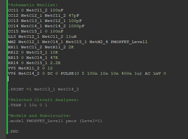
In the coming example, I’ve used the buck converter circuit shown below. This circuit uses a relatively large inductor in the main section (L1), followed by an L-filter on the output to further reduce switching noise. The output capacitor has a snubber resistor to help reduce the strength of the transient response and smooths the output voltage.
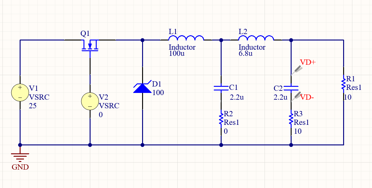
This circuit is intended to step down the input 25 V down to about 6.75 V. In my simulation, I’m going to allow the inductor values to vary by up to 30%, and I’ll perform 15 runs. This large variation would be found in some wirewound inductors and ferrites, and using such a large variation can help you see what the extreme values of ripple and overshoot might be.
The other reason the inductor is the varied component in the is that it is a major determinant of output ripple when the converter is operating in the continuous conduction mode. We could even go a step further and look at the inductor current itself to see how close the inductor current comes to continuous conduction if we really needed to verify the worst-case electrical behavior.
Results
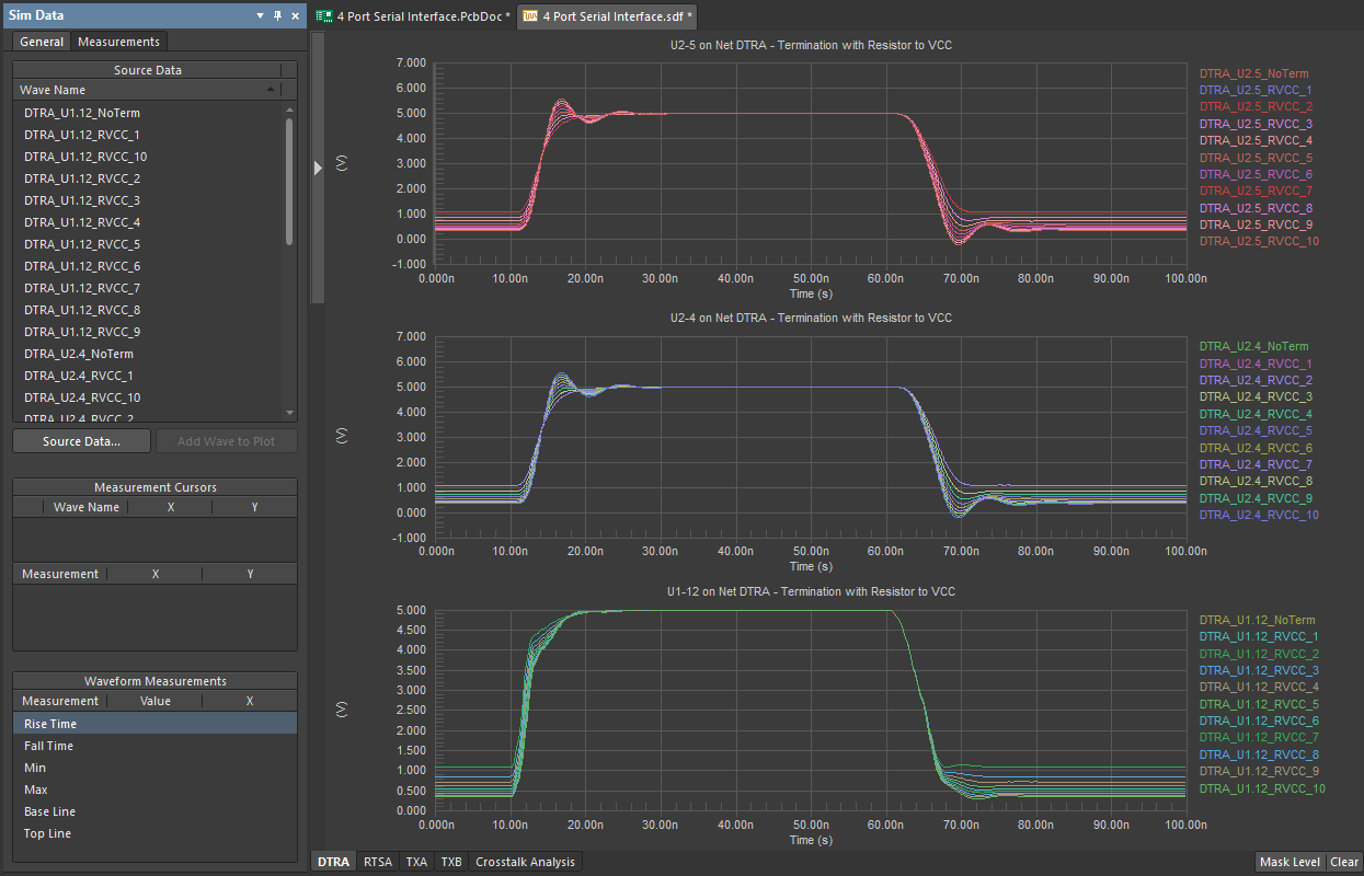
Some initial results showing the transient response given 30% variations in the component values are shown below. From this window, we see that the converter already exhibits some overshoot ranging from 8.37 V to 8.56 V, depending on the values of the inductors. The values for the lower contour (in green, L1 = 91.9 uH, L2 = 6.16 uH) and upper contour (in purple, L1 = 122uH, L2 = 7.64 uH) are marked on the graph below.
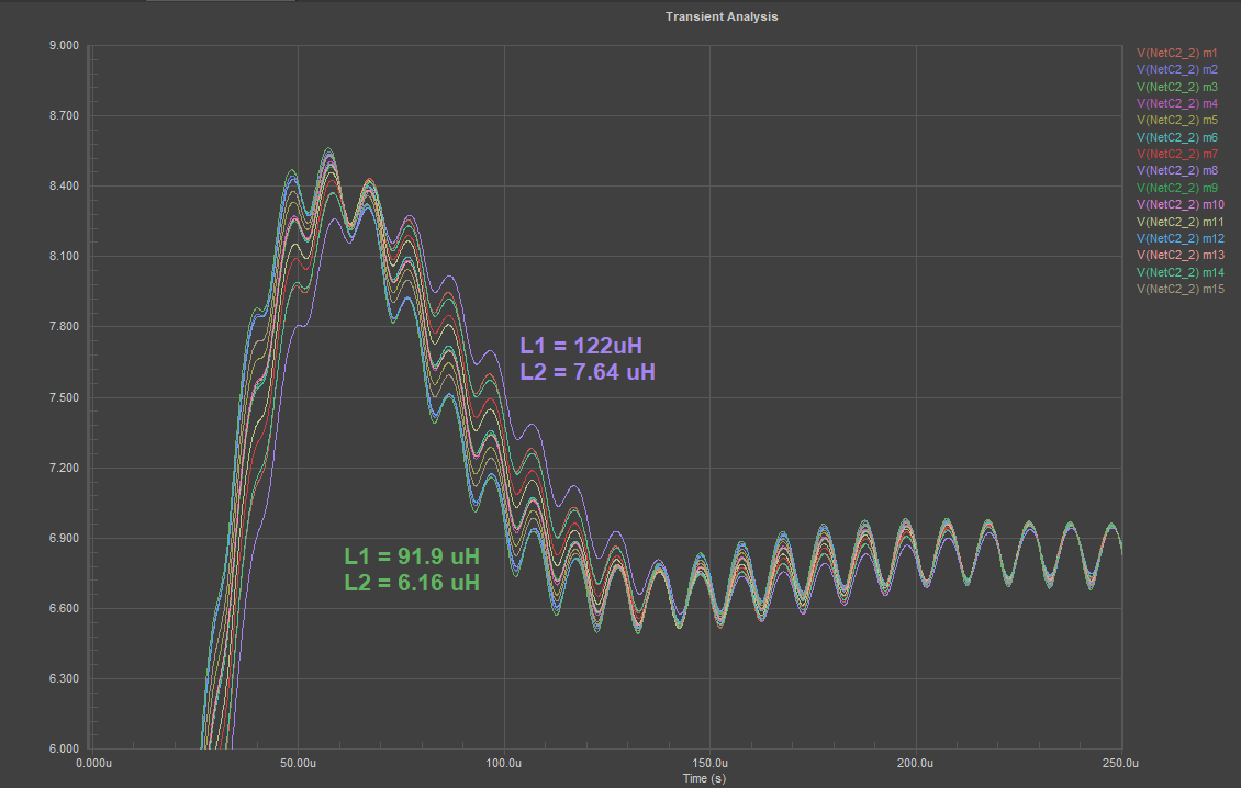
Each curve corresponds to a pair of randomly generated inductor values. From the results, we can clearly see the effects of variations in the inductor:
- There is some variation in the rise time, overshoot, and transient response as the regulator turns on.
- Each possible inductance value produces very small changes in the ripple on the output voltage waveform.
The fact that the output ripple remains so low is encouraging; it means we can rely on this design to output consistent ripple assuming small variations in all other parameters.
Why is the Change in Ripple So Low?
Without looking at the equation for the output ripple as a function of output inductance, it’s natural to assume that a change in the inductance of +/- 30% would produce similarly large variations in the output inductance. However, if we look at the equation for the voltage waveform ripple on the output current for a buck converter operating in the continuous conduction mode, we can see why this is not the case:

Because the inductance value is in the denominator, the effect of those variations is reduced. You can see this by taking a perturbation about the nominal inductor values and looking at how the ripple sensitivity is proportional to any variation in the inductances:

The impact of these variations is reduced by the value of the inductor. In other words, a 30% tolerance for a large inductor will create a much lower change in the output ripple than the same 30% tolerance on a smaller inductor. This behavior is typical when the relationship between some electrical value (current in this case) is nonlinearly related to the component value in question.
In addition, the 3 dB roll-off frequency in the output filter (L2 + C2) is already below the PWM frequency that modulates Q1. The 3 dB rolloff in this filter section is nominally 41.1 kHz, while the ripple frequency matches the PWM frequency of 100 kHz. The ripple will already be filtered significantly, so the resulting variations in the rolloff frequency do not have so much impact on the output ripple.
Statistical Analysis
If you’re going to do Monte Carlo analysis, you may need to do some statistics analysis to really understand the limits of your circuit’s behavior due to random variations in component values. In the graph below, I’ve taken my above transient analysis results and extracted the maximum voltage that occurs during the turn-on phase due to overshoot. I’ve calculated the average and standard deviation to quantify the effects of variations in the inductance values.
To export your transient results in CSV or other data format, use the File → Export → Plot command from the main menu in Altium Designer. You can then import your data into Excel, MATLAB, Mathematica, or other data analysis program.

If we build a confidence interval using our collected data and the above statistical values, 95% of these circuits will exhibit an overshoot ranging from 8.375 V to 8.605 V. If we wanted to perform further analysis, such as worst-case analysis, we could use either of these extreme values to understand circuit behavior.
Reliability Evaluation With Larger Datasets
To evaluate reliability statistically, you might run a much larger number of simulations, so you would have a lot of data points to look at. With more data, you could build a histogram from your extracted measurements and use this to get a probability distribution that defines the circuit’s behavior; you could then use these values to determine the probability that the circuit operates in a totally unacceptable regime (beyond the extreme values in our confidence interval).
Just for fun, I’ve increased the number of simulations performed in this analysis to 100 runs. The transient results with 100 iterations is shown below. From these curves, we can again extract the maximum overshoot voltage during the turn-on phase.

If you export the results into Excel, you’ll now have enough data to create a histogram like the one shown below. The overlaid orange curve shows the cumulative function determined from the binned data; it shows what percentage of the data lies at or below the current bin and can be used as a measure of the expected operating range of this circuit.

The takeaway here is that we have a quick and easy way to check how the circuit performance will vary given component tolerances. If the results are not within our specifications or margins of safety, then the circuit will need to be modified before creating the PCB layout and assembling a prototype.
If you’re interested in running Monte Carlo simulations for your circuits inside Altium Designer®, you don’t need an external simulation package or specialized analysis software. Everything you need to evaluate your circuits and perform reliability simulations can be found inside the schematic editor in Altium Designer. Once you’ve completed your PCB and you’re ready to share your designs with collaborators or your manufacturer, you can share your completed designs through the Altium 365™ platform. Everything you need to design and produce advanced electronics can be found in one software package.
We have only scratched the surface of what is possible to do with Altium Designer on Altium 365. Start your free trial of Altium Designer + Altium 365 today.

About Author
Related Resources


Related Technical Documentation


Take advantage of the world's
most trusted PCB design system.
One interface. One data
model. Endless possibilities.
Effortlessly collaborate with
mechanical designers.
The world's most trusted
PCB design platform
Best in class interactive
routing
View License Options
Thank you, you are now subscribed to updates.