CAN-Bus: Introduction and History

This article is part of a three-part introductory series on the controller area network bus (better known as CAN bus):
- Part 1: An Informal Introduction
- Part 2: The Protocol
- Part 3: Designing CAN bus circuitry
Meta-Introduction to the CAN Bus
Over the past few decades, the industry has consolidated to a limited number of commonly adopted communication buses, from local communication standards such as SPI, I2C, and UART to RS232 and USB that can span a few meters. RS485 and CAN bus commonly operate from a few tens of meters up to a kilometre, and Ethernet can span over tens of kilometres in the form of fiber optical links.
Many of the most common buses are point-to-point, meaning devices are connected in pairs. For example, every computer connected through Ethernet is physically linked to only one other device, usually a switch. Similarly, if you want to connect multiple USB devices to one port, you need a USB hub. A passive three-headed Ethernet or USB cable where three devices communicate with each other cannot exist while respecting the relevant standard.
RS485 and CAN bus are examples of popular buses that allow multiple devices to interact together; CAN bus is the only multi-master bus with widespread adoption. There are many reasons why you should consider CAN bus for your next project. The standard is widely adopted, affordable, absurdly reliable, extremely resistant to EMI (electromagnetic interference), and devilishly clever in its design.
That’s a lot of superlatives.
Moreover, while we transition into an increasingly hyperconnected society, the CAN bus offers a refreshing alternative to the unpredictability and fast technological turnover of WiFi and mesh networks.
History
In the early 1980s, automotive electrical systems were rapidly growing in size, complexity, and cost. Consumers demanded more and more features and increased automation to reach the pinnacles of luxury and modernity.
1982’s popular TV series Knight Rider pushed everyone to imagine what an increasingly digitalized car would look like, a trend that never stopped and continues with Tesla today.
To cut down on the ever-growing mass of intertwined cables and reduce assembly cost and complexity, Bosch started to evaluate existing serial buses for use in cars. None of them fit the requirements, so in 1983 the development of the CAN bus began. The first revision of the standard was officially released in February 1986 at the Society of Automotive Engineers in Detroit.

The CAN bus immediately differentiated itself from every other bus system available by being multi-master, implementing a broad range of error-detection and fault-mitigation mechanisms (including collision-resolution), and identifying data frames not by source and destination but by their content.
In 1987. Intel released the first CAN bus controller integrated circuit, the 82526, and Philips followed shortly thereafter. In 1993, the Bosch specifications were published under the ISO 11898 series of standards.
The first adopters of the CAN bus standard were, curiously, not vehicle manufacturers. Looking back from today, this would be expected due to the current growth of automotive Ethernet, but this was not the case. Instead, northern European industrial giants such as Kone (Finnish elevator manufacturer) and Philips Medical System were some of the first adopters. Philips adopted the standard for their X-ray machines designed in the Netherlands.
Over the late 90s and early 2000s, the CAN bus specifications were expanded with standardized application layers, implementations for safety and real-time applications, and faster data rates. In 2018 Bosch started the development of CAN bus XL, expected to operate at 10 Mbps bandwidth.
Please Do Not Throw Sausage Pizza Away
As electronic engineers with fingertips perennially tainted by colophony, it’s easy to get lost into voltage levels, counting electrons and loudly discussing EMI. Still, CAN bus is, first and foremost, a network protocol.
As such, it’s fundamental to take a look through the lens of the standard OSI (Open System Interconnection) model, composed of seven layers:
- Physical Layer: how the raw bits stream is communicated over the physical medium.
- Data Link Layer: Transmission of data frames between two nodes.
- Network Layer: multi-node network management, addressing, routing, and traffic control
- Transport Layer: Flow control, segmentation-desegmentation, and error control.
- Session Layer: back-and-forth exchanges between two nodes.
- Presentation Layer: Conversion of data between network and application (for example, compression, encryption, and character encoding).
- Application Layer: well, the name says it all.
Hence why “Please Do Not Throw Sausage Pizza Away.”
Similarly to RS-485, the CAN bus operates at the Physical and Data-Link layers, while other protocols such as CANOpen take care of higher-level layers.
Physical Layer(s)
Before dipping the chips into the guacamole, it’s fundamental to understand there are a couple of popular CAN bus standards. What (almost) everyone thinks of when reading “CAN bus” is (apart from drinking coke on public transport) the ISO 11898–2 standard, often called high speed CAN, HS-CAN, or simply CAN.
ISO 11898–2 High Speed CAN
ISO 11898–2 adopts a main twisted-pair bus, terminated at each end with a 120 Ohm resistor; 120 Ohms is also the bus’s characteristic impedance. One of the wires is called CANH, the other one CANL. As you may have guessed from the twisted pair and the widespread usage in EMI-heavy environments, the bus is differential. So far, easy peasy.
It is not always practical to zig-zag the same twisted pair to all nodes of the network; for this reason, the CAN bus bus allows for stub wires of up to 30 cm. If you go over 30 cm, the reflections will start degrading bus performance, as the nodes themselves are not terminated, only the twisted pair.
(Read the 3rd article if you want to know how to cheat this limitation).

Most digital buses are driven high to represent a logic 1 and low to represent a logic 0. This is not the case with the CAN bus, that adopts a state called recessive, describing 1's, and a state called dominant, signifying 0's.
In the recessive state, the termination resistors determine the bus voltages. The transceivers go in a high-impedance state and let the wires live their life in peace and prosperity.
In the dominant state, the transceivers drive the voltages of the CANH and CANL lines apart. The CANH is being driven up at a nominal 3.5V, and the CANL is driven at a nominal 1.5V.

Chronic debugging stress is not good for your health, so here is a little cheat sheet:
| State | Value | Value | Voltage | Determined By | VANH Nominal V | CANL Nominal V |
| Dominant | 0 | Low | CANH > CANL | Transceivers | 3.5 | 1.5 |
| Recessive | 1 | High | CANH = CANL | Termination Resistors | 2.5 | 2.5 |
ISO 11898–3 Low-Speed Fault-Tolerant CAN
ISO 11898–3 is a low speed and fault-tolerant variation of the CAN bus standard. I would love if some prominent engineer were to shorten it as LSFTCAN or CANFTLS, it would truly make a mockery of our over-reliance on acronyms.
There are three main differences between ISO 11898–2 (CAN or high-speed CAN) and ISO 11898–3 (low-speed fault-tolerant CAN): network structure, voltages, and bandwidth.
The low-speed fault-tolerant CAN bus standard reduces the maximum bandwidth from 1Mbps to 125Kbps, and instead of using two termination-resistors at the start and end of the bus, the resistors are distributed on each node.
Distributed termination resistors translate to less chance of one breaking and a higher risk of reflections and lower network speed.
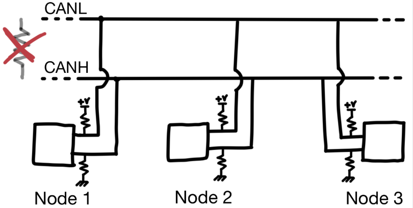
To improve EMI resistance, the voltage swing is approximately double that of high-speed CAN, and the resistors pull CANL high to five volts and CANH low to 0 V during the recessive state. In contrast, during the dominant state, the transceivers invert the voltages, driving CANH high and CANL low.
All this atypical terminology and voltage levels can be very confusing, surely not just because I’m an awful writer, so just remember: the dominant state is the 1 when the name of the lines make sense.
May I be drenched in gold and glory if I ever get this right without a cheat sheet…

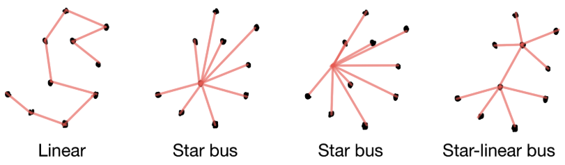
A low-speed fault-tolerant CAN can take a variety of shapes, from a linear bus similar to high-speed CAN to a star-shaped bus, or multiple star-shaped buses interconnected by a linear bus.
SWCAN
There is a third variety of CAN bus network: single-wire CAN, or SWCAN, as specified by SAE J2411. SWCAN is meant for local, low-speed, low-cost operation, and was vigorously promoted by General Motors in the early 2000s. There seems to be some big-company drama going on in the supply chain for SWCAN transceiver ICs, the kind that requires phone calls and meetings to be untangled. Since the SAE J2411 standard has substantial overlap with LIN, you should choose the latter and disregard SWCAN completely.
(If you’re a lawyer, that’s my personal opinion, don’t go suing Altium over it).
Breadboard-CAN
If you need to test the CAN bus with just a few CAN-enabled microcontrollers but no transceivers, for example, to do firmware development while your PCBs are being manufactured, you can use the following trick:

I don’t recommend it, nor guarantee it will work, and you will probably have to lower the speed, but it can be quite useful for testing CAN bus on development boards. The diode should be a small-signal Schottky diode with a low reverse bias capacitance.
Coke or Pepsi?
If you’re just starting with the CAN bus, you should start with ISO 11898–2.
The differences between the two standards are only at the physical layer. The protocol is identical; tools, ICs, and documentation on how to implement high-speed CAN bus networks are more readily available than for the low-speed fault-tolerant variety. If you ever need a low-speed fault-tolerant operation, you can simply upgrade the transceiver and add a couple of resistors.
When Should You Use the CAN Bus?
To no-one's surprise, there are no hard rules to choose CAN bus over any other standard, and the decision will inevitably require a level of engineering finesse.
If the following statements are true, CAN bus is probably for you:
- You need a stable protocol
- The system must have high EMI tolerance
- The bus should be affordable and straightforward to implement (one twisted pair)
- You need a multi-master protocol
- Faulty nodes must not compromise the network
- You need between 100 kbps and 2 Mbps bandwidth
Meanwhile, the following indicate you should choose another protocol:
- Your design is heavily power-constrained
- Your system has just a few nodes and cost is paramount
- You need a lot of bandwidth, for example, for multimedia
How to Prevent Signal Reflections (The Unadulterated Sales Pitch)
In high-speed CAN bus, the ends must be terminated, but this doesn’t mean that signal reflections can’t still happen between the bus nodes. Stub length and node spacing must be carefully controlled; in particular, the stub length should be minimized, the node spacing should be randomized and respect a minimum distance. I have linked at the end of this article a few resources that will explain all the needed calculations.
If you are designing a system with tens, if not hundreds, of nodes, Altium Designer® is not going to be enough by itself to manage the complexity of the whole system. Your system is likely to be composed of hundreds/thousands of pieces intertwined within a mechanical assembly.
You’re likely to be already familiar with advanced mechanical CAD software such as Solidworks, PTC Creo, or Autodesk Inventor. Altium Designer works together with Altium Concord Pro™, to offer you extensive ECAD-MCAD collaboration capabilities. Assuming your project is already saved on the cloud, sharing it with a mechanical engineer won’t take more than a few seconds. In addition, you can import mechanical models of your PCB into any of these three mechanical modeling programs so that you can design your enclosure.
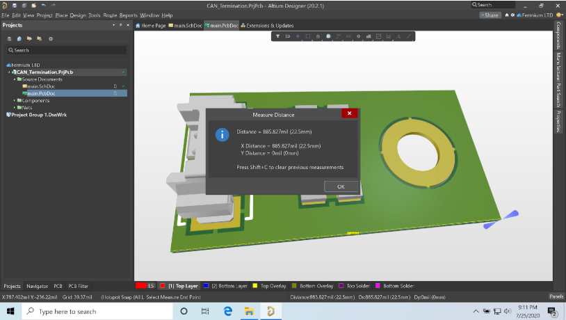
In this example, I have decided to create a quick and easy termination board able to absorb a considerable amount of energy and be easily mounted. The components were added to the schematic with one click through the manufacturer part search.
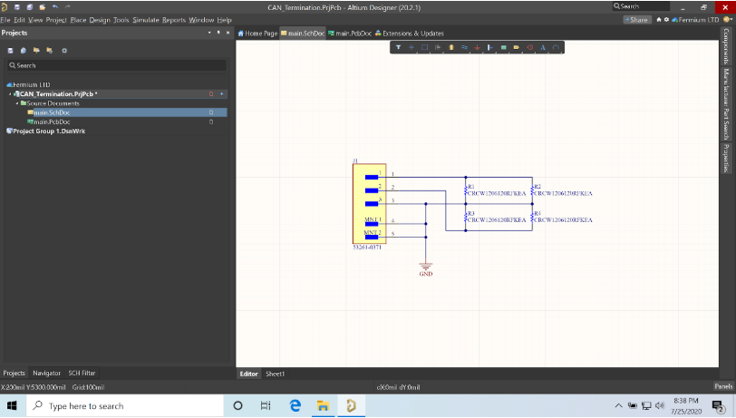
I quickly routed the board. Since everything is integrated into Altium Designer, I didn’t have to fiddle with multiple software, netlists, imports, and exports.
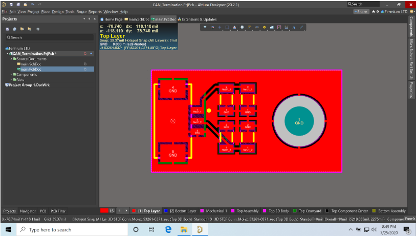
I verified the correctness of the 3D model in Altium Designer using the measurement function (CTRL+M).
I then opened on the Mechanical CoDesigner panel and pushed the design to Concord Pro on Altium 365.

After pushing the MCAD data, Altium Designer immediately asks if you’d like to share your design with a mechanical engineer.
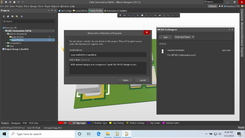
The Mechanical Engineer can then register on Altium 365 following the link provided in the invitation email and install the relevant plugin available for Solidworks, Autodesk Inventor, or PTC Creo.
Further Resources
- Can Bus explained by CSS Electronics
- Texas Instruments SLLA270, “Controller Area Network Physical Layer Requirements”
- Microchip AN228, “A CAN Physical Layer Discussion”
- Analog Devices AN-1123, “Controller Area Network (CAN) Implementation Guide”
- Wolfhard Lawrenz, CAN System Engineering, Springer, ISBN: 978–1–4471–5613–0
- Steve Corrigan (Kvaser), “Minimum distance between CAN nodes”
- Texas Instruments SLLA279A, “Critical Spacing of CAN Bus Connections”
Conclusion
The CAN bus is an intriguing bus that combines the extreme flexibility of a multi-master broadcast protocol with excellent reliability and fault-tolerance. For these reasons, it has seen ever-growing adoption in the industry since the 90s.
Shinier and faster technologies like automotive Ethernet are becoming cheaper, but CAN bus trickles down to the broader electronics industry and shows no signs of slowing down. While CAN bus enables complex electronic designs with tens or hundreds of nodes, such projects are likely to require extensive electronic and mechanical integration.
Altium Concord Pro on Altium 365® enables seamless collaboration between electronic, mechanical, and system design. Would you like to find out more about how Altium can help you with your next PCB design? Talk to an expert at Altium.

About Author
Related Resources


Related Technical Documentation
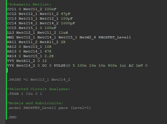

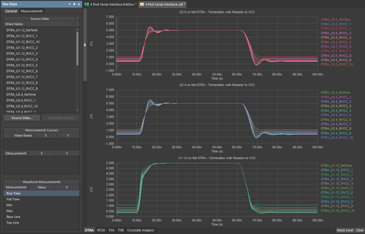
Table of Contents
Take advantage of the world's
most trusted PCB design system.
One interface. One data
model. Endless possibilities.
Effortlessly collaborate with
mechanical designers.
The world's most trusted
PCB design platform
Best in class interactive
routing
View License Options
Thank you, you are now subscribed to updates.