How to Verify Signal Integrity Causality in S-parameters
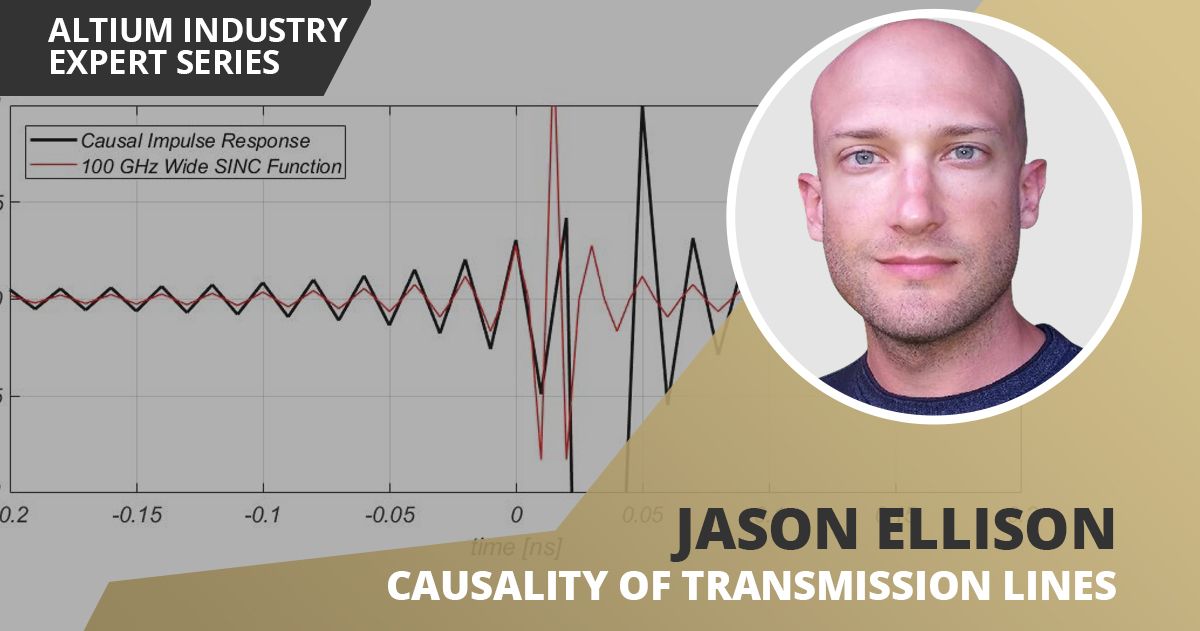
Table of Contents
If you’re doing anything with S-parameters, you’ve run into causality problems. The first time hearing your S-parameters are non-causal is an uncomfortable experience. A customer may say, “your S-parameters fail my causality tool. Please fix them and send me new data. Thanks.” Thanks indeed. After getting that message, you probably went to your resident SI expert, Google, and typed in causality.
When you finish reading what Aristotle has to say about the subject, you still don’t have anything to give to your customer. Many engineers are stuck at this point. Thankfully, there are some simple methods you can use to check and enforce S-parameter causality in your simulations and experimental data.
What is S-parameter Causality and How Do I Check for It?
Causality simply means an effect must happen after a cause. You hit a bell with a hammer, then the bell rings. It would be strange, if not unnerving if the bell rang as the hammer approached it. In systems described by S-parameters, a response must occur after a stimulus. There are three typical stimuli signal integrity engineers analyze: an impulse, a step, and a pulse.
The inverse Fourier transform of an S-parameter is a transfer function for a particular type of signal. For example, Kurokawa's treatment of transmission line S-parameters defines the inputs and outputs in an N-port network in terms of equivalent power, and the S-parameters act like a transfer function for this particular type of signal. Most engineers are more familiar with a standard transfer function in terms of input and output voltage. Regardless of how you define a transfer function (as an S-parameter or filter), every transfer function has an impulse response function.
The first thing to do to check causality with minimal work is to take the inverse Fourier transform of an S-parameter and look for responses before the time of the stimulus (t = zero seconds). Before zero seconds, the system should be at rest, and any non-zero value indicates a causality violation.
I like to say the raw inverse Fourier transform of an S-parameter has a “native rise time”. That means the S-parameter is completely unfiltered and is showing all the information available. An impulse response with native rise time will always seem non-causal because it is bandlimited. This bandwidth limitation means you are effectively taking the inverse Fourier transform of a rectangle function, rect(f), which is a sinc function, sinc(t). Sinc functions look like an impulse response with extra ringing before and after the pulse’s peak. Since there is ringing before zero seconds, the function is non-causal. This implies all S-parameters are non-causal, and yes, that is true by definition. I have an example below in Figure 1 that shows this phenomenon, which is sometimes referred to as “the Gibbs phenomenon” after J. Willard Gibbs.
The black plot is the impulse response of a reflection S-parameter vector, and the red plot is the inverse Fourier transform of a sinc function with the same bandwidth as the impulse response, 100 GHz. You can see the trend identically with magnitude differences. In fact, I normalized these plots to highlight how the ringing matches the sinc function, and the values were actually less similar than I have shown. Therefore, you cannot simply subtract the sinc function from the impulse response to get a causal response.
Instead, apply a windowing function before applying the inverse Fourier transform to get rid of the ringing. A windowing function in the frequency domain is a filter that removes high-frequency content from the transfer function. In the time-domain, a windowing function enforces the periodic nature that is required to perform the discrete Fourier transform of the time-domain function with minimal distortion. There are many windowing functions to choose from. Here are some examples.
Triangle Function
where N is the number of points, and L = N + 1.
Sine Window
Where,
N is the number of points.
Blackman Window
Where,
a0 = 0.42,
a1 = 0.50, and
a2 = 0.08.
In the example below, I applied the Blackman windowing function to the same impulse response shown in figure 1 compared to the same sinc function. This time, the response is clearly causal with no artifacts from the bandlimited spectrum.
You can use this technique to make sure your plots do not have false non-causal artifacts from converting from the frequency domain into the time domain. However, this technique does not fix your S-parameters. It is only so you can visualize the effect and see if a causality violation is truly there.
A Common Source of Non-causal S-parameters: Ghost Limbs
De-embedding is the most common reason for non-causal S-parameters. Eric Bogatin, signal integrity evangelist, calls the phenomenon “ghost limbs.” It is where the fixture has been de-embedded, but the fixture seems to still be present before zero seconds. The impedance plot below in figure 6 is an example of ghost limbs. When the Blackman windowing function is applied to this S-parameter in the frequency domain before applying the inverse Fourier transform, non-zero behavior is still observed before zero seconds.
The easiest way to fix this problem is to enforce causality by definition. You simply multiply the impulse response with the unit step function - see Figure 7. This, by the way, is the same thing as applying a Hilbert transform. Doing this and enforcing passivity (another future blog) will alleviate most of your problems with customer S-parameter quality complaints.
To help you understand what is going on here, I placed a workflow diagram below in Figure 8 showing a simple process of enforcing S-parameter causality.
Who Cares if the S-parameters are Non-Causal?
I think it’s a fair question. When you read about causality in textbooks, it is in the context of linear systems. In its simplest form, a linear system satisfies the principle of superposition and homogeneity. Furthermore, linear systems must be causal to operate in real-time. If a system is non-causal, it cannot be used for system analysis, which is the core reason why causal S-parameters are important. SerDes vendors need causal channels to accurately predict the performance of their products with internal tools. For the rest of the signal integrity world, we need causal S-parameters for tools like ADS, Channel Operating Margin (COM), Seasim, and (my favorite) PyBERT. These tools help us predict the expected outcome of a link with a given silicon technology.
The result of using a non-causal S-parameter in a simulation tool is false performance degradation. A few years ago, I found this when I was evaluating cable assemblies against the IEEE 802.3 100GBASE-CR4 specification. That specification uses COM as a normative metric, and I could not get my simulated cable assemblies to pass. This was a big deal because I couldn’t convince my management my design worked without having models that pass the specification. My loss was within the standard limits, and all of my S-parameters were passing the informative masks. The channel contained the module compliance board (MCB), the connector, the cable assembly PCB, and the raw cable (see Figure 9).
I created the MCB fixture models with Keysight AFR, found the connector model on a connector company’s website, and created all other models with a commercial 3D EM solver. Piece-by-piece, I looked for the problem. Finally, I used a measured cable instead of the modeled cable. I didn’t think there would be a difference since the cable’s measured S-parameters’ magnitude and phase looked almost identical to my model. Still, to my surprise, my simulations suddenly started to pass.
I didn’t understand the root cause at the time, but this was a real wake up call for me. I knew proper S-parameter causality and modeling could literally make or break a design. Years later, I found the proper way to do RLGC generation for causal transmission lines. Next, I’ll show you a tell for non-causal models that you can find yourself. The plot below in Figure 10 shows impulse responses of ten-inch stripline trace models: one causal, the other non-causal.
The first thing to note is the impulse response doesn’t have an obvious problem: the response before zero seconds is zero. The tell for the non-causal response is the shape. It appears as if there is a mirrored image of the intersymbol interference (ISI) upon the time where the impulse peaks. In contrast, the causal response has a sharp rising edge, and the ISI exponentially falls to zero. While the non-causal response appears to have more signal, the channel results show its quality is clearly worse. I have the channel operating margin results and contributions below.
Causal Results
COM = 8.47 dB
ISI variance: 0.49 mV
Non-Causal Results
COM = 7.55
ISI variance: 0.71 mV
Percentage-wise, it doesn’t seem too bad. The ISI is 15% vs. 10% non-causal to causal. However, when you look at ISI’s noise figure, you see there is 45% more ISI in the non-causal trace! In most systems I have been exposed to, customers push the limits of what the hardware can do, and non-causal transmission line models will falsely tell system designers their design is faulty when it is not.
I’m going to quickly tell you how you can ensure the models you’re producing are causal. First, make sure your dielectric properties are frequency-dependent and causal. The best way to do this is to use the Infinite Pole Model by Djordjevic et al. This method is most clearly explained in Hall and Heck’s Advanced Signal Integrity for High-Speed Design. Second, if you are doing RLGC models, make sure all parameters are frequency dependent. As long as you are modeling with frequency-dependent dielectrics, R, G, and C are easy. L is usually the problem. If you are finding your L is not frequency-dependent, try this formula, and it may fix things. However, results may vary.
Final Thoughts
Try not to beat yourself up when you are faced with an S-parameter causality problem. The problem is still prevalent in the industry, even when tier 1 tools are used. If billion-dollar companies are having trouble, I guess you’re in good company! Instead, try to think of it as an opportunity for improving your Fourier transform skills and signal integrity know-how.
The silver lining for component vendors here is non-causal transmission line models that cause end users to not typically catch serious problems. Most system designers use the heuristic causality check that only catches reflection S-parameter issues caused by ghost limbs, and that problem is easily fixed with the method shown above.
Would you like to find out more about how Altium can help you with your next PCB design? Talk to an expert at Altium or discover how utilizing a PCB Transmission Line calculator makes design easier.


