Monte Carlo Analysis With Transfer Functions in Cascaded Circuits

Pro circuit designers don’t just work with components in parallel and series when they design circuits. One way to build circuits is with circuit networks, which will have input and output ports. What happens inside each network can be analyzed in the traditional way (SPICE, by hand, etc.), but what is important is that the network maps an input voltage/current pair to an output voltage and current pair. Mathematically, this is quantified with a transfer function.

When working on high-reliability designs, one important factor to understand is how variances in one portion of your system propagate through to the output of the system. This is not always intuitive. It requires some mathematical derivations by hand, or it requires some simulations to determine variability in electrical behavior in a system.

In this article, I’m going to show how you can use Monte Carlo simulation data to examine how component tolerances affect the electrical behavior of a cascaded network of circuits. The mathematics involve a few points from probability theory that I think everyone should know, but the end result and the process involved are simple to implement in SPICE and Excel.

Theory: Variances in Cascaded Networks

The goal with the theory I’ll present below is to derive an expression that defines variations in the output voltage from a cascaded network to variations in the individual transfer functions in each network. The variations in network transfer functions are assumed to be due to component tolerances only, although you can easily extend this to cases involving temperature or random noise.

To get started, let’s consider the cascaded network shown below. In this network, we are considering a case where each network has 2 ports (input and output). Expanding to 3 ports is a bit more complex, but we can still use the theory shown here if the other ports are only power inputs that do not vary. Each of these networks in my cascade has a transfer function H.

The relationship between the input and output of the network is shown in Eq. (1). In this equation, the transfer function of the entire network is the product of the transfer functions for each network:

Eq. (1): Cascaded network transfer function definition.

In Eq. (1), we’ve taken advantage of the fact that series cascaded networks like those shown above will have a total transfer function that is the product of all the individual transfer functions. This applies for a wide variety of circuits that are constructed as 2-port networks. Now, we can examine the statistical variations in the transfer function for a given tolerance value for components.

Variations in Transfer Functions

The component tolerances in each network will create some variation in the transfer function in each network. We now want to define the variance in the transfer function.

Eq. (2): Transfer function for each network defined in terms of a constant portion (mean) and a random portion (standard deviation).

In Eq. (2), Hi is a random variable that is related to the random variation in the transfer function for network i (ẟHi). In order for this expression to be true, the distribution ẟHi must allow for this type of linear transformation. In general, this is true for Gaussian distributions and uniform distributions, so it is valid in the two major cases often considered in Monte Carlo simulations.

We have not linked ẟHi to component tolerances with a specific equation. However, if you know the tolerances for all components in a circuit network, you can determine ẟHi with a Monte Carlo simulation. Simply set up a simulation for the individual network Hi, and run a Monte Carlo simulation to determine the variance in the transfer function ẟHi.

Variations in Output Voltage

Now that we’ve defined random variations in individual transfer functions, we can define the variation in the output voltage by applying the same linear transformation shown in Eq. (2) to the transfer function product in Eq. (1). I’ve written this as a product in Eq. (3):

Eq. (3): Variation in output voltage.

Here the output voltage also has a constant portion (mean) and a random portion (standard deviation). In other words, Vout is now a random variable that is related to a product of random variables. The mean output voltage is the constant term on the right-hand side:

Eq. (4): Mean output voltage in terms of the mean values of the transfer functions making up the cascaded network.

From this it should be clear that the product of transfer function means is the mean of the total network’s transfer function:

Eq. (5): Mean value of the transfer function for the entire cascaded network in terms of mean transfer function values for individual networks in the cascade.

If we expand the product in Eq. (3), we will have an expression that contains products of multiple ẟHi terms, Hmean, and the variance in the output voltage. At this point, we wil take an approximation that products of any ẟHi terms are very small and can be ignored. This is perfectly acceptable given common component tolerances, even when they reach as high as 20%. I’ll leave the intermediate steps to readers, but you will arrive at the following equation:

Eq. (6): Output voltage in terms of transfer function means and random variations.

This may not look like the final answer, but Eq. (6) does tell you everything you need to know about the random behavior in the output voltage given some variances in the transfer functions! Here we have a random variable (Vout) defined in terms of a linear combination of random variables (the set of ẟHi terms). From multivariate probability theory, we know that the standard deviation of this sum is equal to the quadrature sum of the ẟHi terms. In other words, the standard deviation in Vout is:

Eq. (7): Standard deviation of output voltage in terms of transfer function variances.

In this equation, the st.dev operation refers to standard deviation, and the Var operator refers to variance. With Eq. (7), we can develop a simulation process for relating variations in output voltage to the variations in transfer functions in our cascaded network.

The Process

Now we can develop a process for determining the output voltage variance in terms of the transfer function variance. To do this, your primary tool will be Monte Carlo simulations and a simple statistical analysis program like Excel:

1. Take your cascaded network circuit design and divide it into individual 2-port networks.
2. Run Monte Carlo simulations for each of the networks in #1.
3. Take the data for each network and calculate the transfer function for each Monte Carlo run.
4. Calculate the mean of the transfer function results for each network.
5. Calculate the standard deviation for each transfer function in #3 to get  ẟHi for each network.
6. Use results from #4, #5, and Eq. (7) to get the variation in the output voltage.

Based on the number of data you used in this process, you can go one step further and get a confidence interval for your results.
Example Calculation
Why go through all of this trouble with individual transfer functions? To see why, let’s look at an example.

Suppose you have three circuit networks with different component tolerances (1%, 5%, and 10%) and you have already gone through the above process to determine the variation in each network’s transfer function. Suppose those component tolerance values translate into the example variances shown in the graphic below. Using Eq. (7), we can predict the variation in the output voltage for this hypothetical network:

Example standard deviation of output voltage calculation for known component tolerances and variations in transfer functions.

A 13.63% variance might be excessive, it all depends on the application. From this, we can make a judgment as to whether certain groups of component tolerances should be reduced.

Now let’s say that the output voltage variation is unacceptable for our application, and we want to get a smaller variation. We decide to swap the 5% tolerances and 10% tolerances for 1% tolerances. Without running any new simulations, we immediately know what the output variation will be. For a linear circuit, reducing the tolerance by a factor 10 should reduce the transfer function variance by a factor 10, and so on for other reduction factors. We would then have the following result:

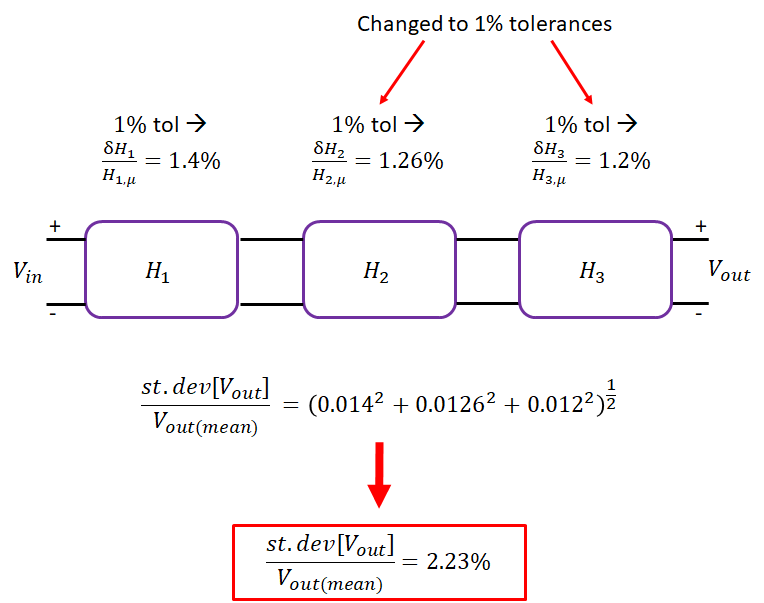
Modified standard deviation of output voltage calculation for smaller component tolerances.

Decreasing the output voltage from 13.63% to 2.23% is a huge reduction, and all it took was a simple component swap. No new circuits needed to be added, no design changes were needed, just select some alternate part numbers. These types of variance reduction steps are exactly what you might need in precision analog applications.

Now let’s say you want to shift your operating frequency. In that case, you can use the transfer function data you obtained from your Monte Carlo simulations to determine how the output voltage will vary at this new frequency using the same calculation.

Summary and Comparison

By knowing how variance in different cascaded networks add to give you a total variance in output voltage, you can directly determine how the output voltage will vary if you do any of the following:

• Swap out components in a network for parts with tighter tolerances
• Swap out a network for a totally different network
• Add an additional network into your cascade

The perturbation method shown above is only applicable to series-cascaded filters or amplifiers. If you have parallel networks, their transfer functions add together, making the variance analysis shown above much easier. Also, you could use this idea to derive a variance expression for combinations of series and parallel networks. No matter how you arrange circuit networks to get a variance expression, the same simulation and analysis method shown above applies.

If you’re interested in running Monte Carlo simulations and transfer function calculations for your circuits inside Altium Designer®, you’ll find these simulation tools built into the SPICE engine in the schematic editor. Once you’ve completed your PCB and you’re ready to share your designs with collaborators or your manufacturer, you can share your completed designs through the Altium 365™ platform. Everything you need to design and produce advanced electronics can be found in one software package.

We have only scratched the surface of what is possible to do with Altium Designer on Altium 365. Start your free trial of Altium Designer + Altium 365 today.