Pole-Zero Analysis and Transient Analysis in Circuit Design

As part of circuit design, it is always advisable to perform some circuit analysis in the frequency domain, time domain, or Laplace domain to understand circuit behavior. The time domain and Laplace domain are related in one area: the transient analysis, where we look at what happens to a circuit as it experiences fast changes in its excitation. From looking at a transfer function in the Laplace or frequency domain, it may not be obvious what the transient behavior is.

Pole-zero analysis involves decomposing the transfer function for a linear time-invariant circuit to determine the rate at which its transient response decays. Eventually, the circuit reaches equilibrium and exhibits its steady state behavior. While this can be viewed in the time domain with a transient simulation, these simulations can take a lot of time and must have the correct time resolution setting to achieve accurate results. Pole-zero analysis is a fast alternative that operates in the Laplace domain, and it's simple to access this through the SPICE simulation engine in Altium Designer.

Pole-Zero Analysis in Transient Analysis

Pole-Zero analysis enables you to determine the stability of a single input, single output linear system, by calculating the poles and/or zeros in the small-signal AC transfer function for the circuit. The DC operating point of the circuit is found and then linearized, small-signal models for all non-linear devices in the circuit are determined. This circuit is then used to find the poles and zeros that satisfy the transfer function.

The transfer function can either show voltage gain (output voltage/input voltage) or impedance (output voltage/input current). The traditional approach is to show voltage gain. In Pole-zero analysis, we actually bypass the transfer function to get three important pieces of information:

• The damping constant for the transient response
• The natural oscillation frequency for the transient response
• Excitation frequencies that exhibit zero response

If you are familiar with transfer functions and Laplace transforms, then you are already familiar with the idea of poles and zeroes in a circuit’s response. Pole analysis is based on calculating the damping constant and oscillation frequency in a circuit, effectively showing you maxima in the transfer function. As most circuits are purely involve first order or second order derivatives of the charge in the circuit, the output from a pole-zero simulation will generally reveal two possible poles in your circuit. Higher order circuits may have many more poles and/or zeroes (3 or more). Calculating these values by hand directly from the transfer function for very complex circuit can be difficult as it may require solving a third degree or higher polynomial, and the problem can become intractable.

Pole-zero analysis automates this process for you. The example below shows the output from pole-zero analysis. If we look at the graph, we see there are two poles and one zero. Note that the real parts of these values are negative. The two poles are complex conjugates of each other (as they should be), and the zero lies along the real axis.

Example and Setup

An example circuit that can be analyzed with pole-zero analysis is shown below

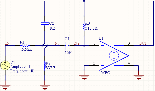
In Altium Designer, pole-zero analysis works with resistors, capacitors, inductors, linear-controlled sources, independent sources, diodes, BJTs, MOSFETs, and JFETs. Transmission lines are not supported but they could be modeled in the schematic as a lumped element circuit as long as the RLCG values are known. The above circuit is assumed to have the following properties:

• Time-invariant circuit element values
• E1 is operating in the linear range (no railing)

Pole-zero analysis is set up on the Analysis Setup & Run dropdown area in the Simulation Dashboard (scroll down to #3, click the Pole-Zero Analysis entry in the Advanced section). An example setup for this analysis type is shown in the image below:

A pole-zero analysis calculation requires the following parameter definitions:

• Input Node - the positive input node for the circuit.
• Input Reference Node - the reference node for the input of the circuit (Default = 0 (GND)).
• Output Node - the positive output node for the circuit.
• Output Reference Node - the reference node for the output of the circuit (Default = 0 (GND)).
• Transfer Function Type - defines the type of ac small-signal transfer function to be used for the circuit when calculating the poles and/or zeros. There are two types available:
• V(output)/V(input) - Voltage Gain Transfer Function.
• V(output)/I(input) - Impedance Transfer Function.
• Analysis Type - allows you to further refine the role of the analysis. Choose to find all poles that satisfy the transfer function for the circuit (Poles Only), all zeros (Zeros Only), or both Poles and Zeros.

The method used in the analysis is a sub-optimal numerical search. For large circuits it may take a considerable time or fail to find all poles and zeros. For some circuits, the method becomes "lost" and finds an excessive number of poles or zeros. If there is non-convergence in finding both poles and zeros, refine the analysis to calculate only poles or only zeros.

The simulation results are displayed on the Pole-Zero Analysis tab of the Waveform Analysis window.

Example output from pole-zero analysis as part of transient analysis

Interpreting the Results

The values on the imaginary axis are natural frequencies and the real axis denotes the transient decay rate (damping constant). The location of the poles tells us four things in transient analysis.

1. The real part of the pole is the damping constant in the circuit. In the above plot, the real part of the poles is negative, meaning the transient responses will decay over time.
2. The imaginary part is the frequency at which the transient response will oscillate (about 1 kHz). In this case, the transient response will produce an underdamped oscillation. Note that, if the poles were located on the right half of the graph (i.e., the real part of the poles was positive), then this system would be unstable with diverging limit cycle, and the transient response would grow over time.
3. Poles lying at x = 0 are resonant frequencies that correspond to harmonic driving with an AC signal.
4. The zeroes of a transfer function refer to specific frequencies that produce a zero output in the circuit.

If you complete pole-zero analysis and you find that your circuit exhibits an undesired response (i.e., an underdamped response in an impedance matching network), you can iterate through different component values in your circuit to determine the component values that produce the desired response. This allows you to critically damp the response in your circuit such that you can eliminate overshoot/undershoot.

When you work with the circuit simulation tools in Altium Designer^®, you won’t have to conduct transient analysis by hand. The industry-standard layout and simulation tools are ideal for circuit design, circuit simulation, PCB layout, and much more. These tools are integrated into a single platform, allowing them to be quickly incorporated into your workflow.

Contact us or download a free trial if you’re interested in learning more about Altium Designer. You’ll have access to the industry’s best layout, simulation, and data management tools in a single program. Talk to an Altium expert today to learn more.