DFSI: Stripline Differential Impedance Calculation Made Easy
Table of Contents

As a PCB designer, you may hear your signal integrity overlords dictate controlled impedance with a specific value and tolerance. As someone who has requested these things, I know designers have trouble with implementing this in their trace geometry. This article details what impedance is, how it is calculated, and a practical way for PCB designers to determine the proper geometry for their application.
When designing high-speed serial circuits, you need to control trace impedance. Impedance is the instantaneous ratio of voltage to current. Instantaneous here means it can change anywhere in the trace instead of considering the trace as a whole. A controlled impedance is where the impedance of the trace is consistent through the entire channel, and there is special consideration for trace geometry when the board is fabricated. The impedance is based on the cross-sectional geometry of the trace. In stripline specifically, the trace width (w), the trace thickness (t), the distance between ground plates (b), and the relative permittivity (better known as DK). When considering differential traces, add the space between traces (s) to this list.
Figure 1. Cross-section geometry of a stripline trace.
If you control impedance, you place a tolerance in the fabrication notes. Typical impedance tolerances are 10% and 7%, and can go as low as 5% or 2% in the extreme cases. The board house achieves these tolerances by observing how their process affects impedance historically, and usually run a test to predict the best geometry. In the end, what a PCB designer cares about are these starting dimensions. So, how do you calculate impedance using these inputs?
Commonly, you calculate impedance from either finite difference (FD), numerical analysis, or conformal mapping. FD numerical analysis and conformal mapping start by finding the voltage, V, by satisfying this Laplacian equation.
Using this equation, you find the voltage based on the geometry. You can then use this value to define the electric field and the charge density. Finally, you can put it all together to find ratio of potential charge to get the capacitance per meter. This is always the primary goal of impedance calculations. Plug that into the equation below and you get impedance!
In the case of FD, a rectangular grid represents the geometry. The intersection points of the grid are the nodes used for calculation. Each node has a voltage that is either known or unknown. A differential equation is solved by using a finite difference equation (forward-difference, central-difference, Taylor series, etc.) to find the voltage at each unknown node.
Usually, a technique called the Crank-Nicolson method is implemented because it is both accurate and unconditionally stable. The method can be further refined by how the calculation is completed. It can either use the band matrix method, a sparse matrix that is relatively easy to solve using an inverse, or an iterative method such as successive over-relaxation or Jacobi that seeks equilibrium.
When voltage is known, change is found by implementing a discrete version of Gauss’s Law without considering the dielectric, Q0, and with dielectric, Q.

Then, you solve the capacitances for each of the above Q’s assuming the voltage difference between conductors is 1.

Finally, impedance is found with
Where, c is 3e8 m/s. Details of this methodology are found in [1].
Does all this sound confusing? Well, it is, and this is the simplest and most comprehendible numerical method used for solving an electromagnetic problem. Clearly, this is more of a physics problem than an engineering problem, and I think this is why engineers focus on using third-party tools instead of solving these equations themselves.
Next, I’ll go over an overview of the other method of solving impedance, then I’ll present something practical that gets around all of this.
Conformal mapping finds an analytical solution to the same problem, and it is difficult to do. In fact, the author of Microwave Engineering, David Pozar, writes “the resulting solution, however, involves complicated special functions” when describing the solution presented in the chapter including trace analysis [2]. If you have delved into Pozar’s writing, you know it’s bad when he says the math is too complex to present. Then again, maybe that was just the solution presented by Howe [3]. In any case, the good news is that the work has already been done. In fact, every geometry worth solving with conformal mapping has been solved, and that includes striplines! The single-ended stripline equation presented by Cohn is actually quite simple [4].

Where Cf’ is the fringing capacitance.
The conformal mapping solution for differential traces is significantly more involved [5]. At risk of sounding like Pozar, it is too cumbersome to write it in a blog. I don’t think that’s a bad thing, because I like to keep things simple. Remember, in the end, we just want the inputs above presented so we can create the right geometry for our boards. Let’s get the easy stuff out of the way first.
If you’re routing stripline traces, you’re doing it with half-ounce copper. An argument could be made to use one-ounce or quarter-ounce copper instead. One-ounce has the allure of promising lower loss from the increased surface area. However, your returns are diminished when the impedance is out of control from the etch-factor related to one-ounce copper. Further, it is expensive to use one-ounce, because no one stocks it. A similar story can be told for quarter-ounce. It has the allure of improved impedance control, but the loss and cost are increased. So, I’m assuming half-ounce copper here: t = 0.015mm.
Next is DK. When I think of DK, I think it comes with a chosen material. Since chosen PCB laminates will vary, this seems to be an important input. However, the domain can be limited to something practical. In this case, I’m going to limit the domain to 3 to 4. From experience, materials suitable for high-speed serial application are in this range.
Now we’re down to width (w), ground plate separation (b), and space between traces (s). Usually, trace width and space are equal or the space is a little smaller than the width. I’m sure it has happened, but I’ve never encountered an application where the space was greater than the width. So, I’m going to make the assumption that space is equation to width: s = w.
Almost done. The ground plate separation (b) is easily incorporated by using an input of width to separation ratio, U. It turns out, this ratio is everywhere in the equations, and it makes it really easy to simplify the analysis.
Here is the final product, a chart of DK vs U for three common impedance values.
Figure 2. Chart of DK vs U for three common impedance values
So, you start with a material; that will give you DK. Then you can either a) pick a trace width and let that define your ground separation, or b) pick your ground separation and let that define your width and spacing. The latter is probably more convenient unless you have a density requirement.

For those who would like to pick an exact number, I have a table for you!
|
DK |
U for Z-Diff = 85 |
U for Z-Diff = 90 |
U for Z-Diff = 100 |
|
3.0 |
0.619 |
0.560 |
0.451 |
|
3.1 |
0.602 |
0.543 |
0.434 |
|
3.2 |
0.586 |
0.527 |
0.418 |
|
3.3 |
0.570 |
0.511 |
0.402 |
|
3.4 |
0.555 |
0.496 |
0.386 |
|
3.5 |
0.540 |
0.481 |
0.371 |
|
3.6 |
0.525 |
0.467 |
0.356 |
|
3.7 |
0.511 |
0.453 |
0.341 |
|
3.8 |
0.498 |
0.439 |
0.326 |
|
3.9 |
0.485 |
0.426 |
0.312 |
|
4.0 |
0.472 |
0.413 |
0.298 |
I’ve been using this technique to design traces for quite a while, and I’ve been surprisingly happy with the results. So much so that I don’t bother to use a 2D solver anymore for picking trace geometries!
Lately, there has been a buzz in the SI community about Altium Designer® improving their impedance calculator utility with the new improvements in version 19. Someone on the SI list did a quick check, and Altium Designer was getting results very close to ADS.
If you have Altium Designer 19, and want to use the impedance calculator within, here is a quick how-to for you:
-
From the toolbar: Design → Layer Stack Manager
-
Click on the impedance tab at the bottom of the Layer Stack Manager
-
Click on one of the signal layers
-
View the impedance panels from the toolbar: View → Panels → Properties
You’ll see something like this:
Figure 3. Altium Designer 19 Impedance Calculator
I used the value from the table for DK = 3.2 and b = 14 mils; that yielded w = 7.378 mils. You can see Altium Designer’s impedance calculator agrees within 5% which is easily good enough for any board house to obtain proper impedance control, and it is an extremely fast process.
As I stated above, the assumption here is that space equals width, and that is not always the case. If there is a demand for a different width:space ratio instead of 1:1, I’ll add it to the next blog. Another possibility is to do the same thing for microstrip. Just let me know what you would like to see in the comments!
All plots were generated using Octave version 5.1.0.
Have more questions? Call an expert at Altium or read more about incorporating impedance calculations into your design rules with Altium Designer®.
References:
[1] M.N.O. Sadiku, “Numerical Techniques in Electromagnetics with MATLAB”, Third Edition
[2] D. Pozar, “Electromagnetic Theory”, in Microwave Engineering, 3rd ed, New York, Wiley
[3] H. Howe, Jr., Stripline Circuit Design, Artech House, Dedham, MA, 1974
[4] S. B. Cohn. “Characteristic Impedance of the Shielded-Strip Transmission Line,” IRE Trans. Microwave Theory and Techniques, Vol. 2 Iss. 2, July, 1954, pp 52-57
[5] S. B. Cohn. "Shielded Coupled-Strip Transmission Line," IRE Trans. Microwave Theory and Techniques, Vol. MTT-3, October, 1955, pp. 29-38.
About Author
Related Resources


Related Technical Documentation

Take advantage of the world's
most trusted PCB design system.
One interface. One data
model. Endless possibilities.
Effortlessly collaborate with
mechanical designers.
The world's most trusted
PCB design platform
Best in class interactive
routing
View License Options
Thank you, you are now subscribed to updates.