It’s Your Loss: Determining And Controlling Loss In The PCB Design Process

When it comes to designing a high-speed PCB, we always have to factor in the dynamic of signal loss. And, there are lots of areas where loss can occur. Accounting for all of these aspects of loss can be a challenging and time-consuming task as too much loss can prevent a high-speed PCB from functioning properly. This article will address the various aspects of loss, how they factor into the PCB design process, and how loss can be effectively determined and controlled.
A Lot of Information and a Little Bit of History
To begin, loss comes from three places:
• Loss in the resin
• Loss in the glass of the cloth
• Loss in the copper
Laminate or Dielectric Loss
Just to review, loss is a function of both frequency and the length of the transmission line. When it comes to high-speed PCB design the thing to remember is the lower the loss the better, and loss changes with frequency. The higher the frequency, the more loss there is in any given material. The reason that loss exists and gets larger with frequency is that the changing electromagnetic field (RF field) causes the molecules in the dielectric to vibrate. The faster they vibrate, the more loss there is.
Loss really comes into focus with the resin system or the laminate which is a composite of the resin and the glass. Note: the term laminate loss is used interchangeably with dielectric loss.
Part of the laminate selection process focuses on the loss tangent tan(f) or dissipation factor (DF) of any given material. The tan(f) is a measure of how much of the energy in an RF signal is lost in the dielectric of the PCB and it is one of the properties of a piece of laminate that is provided by the laminate supplier.
Different Styles of Glasses
Historically, manipulating the loss in laminates involved two things—modifying the glass or modifying the resin. Nearly all glass used to make the cloths for PCBs is E (electrical) glass. It is formulated for easy weaving and adhesion of the resin to the glass.
The challenge is that E glass has a relatively high loss tangent. Some years back, a couple of glass manufacturers modified the glass formula to create S (strength) glass which has a lower loss than E glass. Early on, almost anyone going up the speed curve chose a laminate made with S glass. The problem was that there was only one source for S glass (Nitobo) and it was located in Japan. Additionally, there was only one widely available laminate, Nelco’s original 4000-13 SI, that contained S glass. Overnight the entire industry changed when the earthquake and tsunami hit Japan in 2011 and S glass went entirely away.
All of the other laminate suppliers modified their resin systems such that their laminates became low loss so the need for S glass disappeared and it is rarely used. The real benefit of this is that the sole-source problem that was associated with S glass has gone away.
Copper Loss and Skin-effect loss
Once the resin systems had been successfully addressed, the industry next turned to looking at loss in copper.
Copper loss has three components:
• The wider the trace, the more surface area there is.
• The roughness of the copper
• The basic conductivity of the copper
In contrast to dielectric loss, copper or skin-effect loss is associated with the current that flows into conductors and crowds into a thin layer near the surface at high frequencies. Similar to dielectric loss, skin-effect loss gets larger as frequencies go up. It is compensated for by increasing the width of the traces to create more surface area. A wider trace means lower skin-effect loss. In designing a PCB stackup, tradeoffs between skin-effect losses and dielectric losses are made by determining which dielectric/laminate to use and how wide the traces on the PCB will be.
Historically, copper was made rough so that it would bond to the laminate. The problem was that this rough copper produced quite a bit of loss. But, because loss was not an initial area of concern, the roughness of the copper was not an issue. Figures 1 and 2 show the difference between smooth and rough copper. Figure 1 is the smooth copper and Figure 2 is the rough copper.

Figure 1. Very Low Profile Copper Foil (VLP)
Figure 2. Reverse Treat Copper Foil (RTF)
To address the problem of loss and copper roughness, the industry pushed for very smooth or very low profile (VLP) copper. The problem was that it did not bond well. Eventually, a whole new set of chemistry was developed to make the smooth copper bond to the resins during lamination.
However, no matter how much effort has been put into making the copper smooth, it still has irregularities—peaks and valleys—which contribute to loss. When the copper was being made rough to ensure that it would bond to the resin, the height of the roughness was 8 or 10 microns. The smooth copper is 2 microns, but it still contributes to loss. There has to be some way to model those 2 microns, and there are three different math models that enable that process.
In terms of the conductivity of copper, all copper is plated so it is a constant across the industry and is not a variable relative to loss.
Now, there are two loss elements left that the engineer needs to manipulate: how much surface there is (trace width), and how rough the surface is. There are two simulators of choice which are primarily used to model loss: Polar’s SI9000, and Mentor’s Hyperlynx with the GHz package. Note: The three accepted models for surface roughness are in the Polar tool.
The Good News and the Bad News
Not so many years ago (in the overall span of the history of PCBs), it was difficult to get loss information from laminate companies. In 2011, the testing of materials was done such that the necessary loss information could become known. Nowadays, as a result of the pressure coming from the design community, all the suppliers of low-loss materials, including those offshore, provide good, reliable loss information for their materials.
The Effect of Vias on Path Loss
So, once we got all the material information in place, there came yet another loss design wrinkle that needed addressing. We all assumed that, because of loss, the nets that we needed to worry about were the long ones, but it turned out that it was actually the short ones that were failing. In 2010, IBM published a paper entitled, “Short May Not Be Better”, DesignCon 2010, Steinberger, et al. IBM had built a really big server that contained a lot of 10Gb or faster nets. The concern was that the failures would be the result of these long nets. Instead, the short nets failed because of the reflections off the vias. While both the long and short nets had vias, the long nets had enough loss that they absorbed the reflections from the vias.
Figure 3 illustrates what occurred with the short nets, which failed.
Figure 3. Loss vs Frequency for two 8” (20 cm) Lines, Routed on Two Different Layers
As shown, the red curve has a roll-off as would be expected. When the via went from the device lead to a trace near the bottom of the board and then back up to the lead, the capacitance was distributed along the length of the via. When the via only went down to layer three (the blue curve) and then crossed, the capacitance of the via was “hanging down” such that it caused disastrous loss. If you use a simulation tool and simulate that via, you create a band-pass filter. .3pf is not a big deal until you are at 4-5Ghz. Above that, it can be a huge problem.
The key thing here is that the reflection of the via of the short net is not lost in a lossy line. Rather, If you have to route on a layer near the top of the board, you have to back drill the unwanted capacitance of the via. While doable, this is by no means a cheap proposition. Instead, we recommend the use of the following technique: Put all of the fast traces near the bottom (signal layers) of the board. Note: In a big backplane this approach won’t work. When you have a backplane with nothing but high-speed signals, you have no choice other than to back drill.
Summary
The subject of loss is multifaceted and somewhat complicated. However, with today’s material information supplied by laminate manufacturers and the capabilities of current simulation toolsets, it is possible to predict loss with extreme precision.
Altium Designer® includes signal integrity tools for PCB Designers as well as power integrity analysis tools in a single program talk to an Altium expert today to learn more.
References
-
“High-Speed Signal Path Losses as Related to PCB Laminate Type and Copper Roughness,” Lee Ritchey, John Zasio, Rich Pangier, and Gerry Partida. DesignCon 2013 proceedings.
-
“When Shorter Isn’t Better,” Michael Steinberger, Paul Wildes, Erick Brock, Walter Katz, and Mike Higgins. DesignCon 2010, Track 7, Multi-Gigabit Serial Interconnects, 7-TA3.
-
Ritchey, Lee W. and Zasio, John J., “Right The First Time, A Practical Handbook on High-Speed PCB and System Design, Volumes 1 and 2.”
About Author
Related Resources


Related Technical Documentation

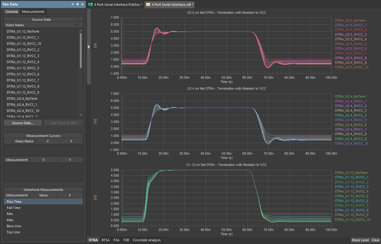

Table of Contents
Take advantage of the world's
most trusted PCB design system.
One interface. One data
model. Endless possibilities.
Effortlessly collaborate with
mechanical designers.
The world's most trusted
PCB design platform
Best in class interactive
routing
View License Options
Thank you, you are now subscribed to updates.