Transformer Theory Made Simple

Transformers can provide very effective signal isolation and are used to manipulate AC voltage and current levels. They can achieve all this with a greater than 95% power efficiency, which is why we commonly see them used in bench power supplies, audio gear, computers, kitchen appliances, and wall-warts. Transformers used for 50/60 Hz power conversion have to be physically larger than those used in wall-warts, and hopefully, after reading this article, you will understand why. However, transformer theory can be unintuitive and, questions like these are commonly asked:

• Will the core saturate when the secondary load draws more current?
• Why won’t my transformer work at 1 Hz or DC?
• Why isn’t my power transformer working at 10 kHz?
• Why does my transformer get hot when there is no load?

Idealized Transformer

This article is intended as a refresher course for transformer theory so, let’s begin with an idealized transformer consisting of two windings wound on a common core. Both windings (red and blue) have the same number of turns, i.e., they have a 1:1 turns ratio:

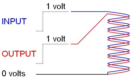
This is an idealized transformer. For a real transformer, if we applied a step increase of 1 volt to the primary, the secondary would produce 1 volt but only for a limited period. This is because transformers are AC devices, and they don’t deal with low frequencies very well. 

However, as this is an introduction and we are talking about an idealized transformer, it is justified to take a few small liberties. Later on, a more realistic picture will emerge. For now, we are just considering an idealized model.

The blue winding is called the primary winding, and the red winding is called the secondary winding. When we apply 1 volt to the primary (blue) winding, we see 1 volt appear on the secondary (red) winding. To understand why this happens, we need to analyze the current that flows into the primary winding:

When we apply 1 volt, the primary current starts at 0 amps and rises linearly with time. If the 1 volt input was maintained on the primary, the current would continue to rise but would soon reach a value that a “real-life” power source couldn’t sustain as the winding is a short circuit for DC. However, we are talking about an idealized transformer at this moment.

The primary current will change (Δi) with time (Δt) at a rate  determined by this formula:

• is just a way of saying “the change of something”
• Δi means “the change of current”
• Δt means “the change in time,” and hence:
• Δi / Δt means “the rate at which current is changing with time”
•  V is the applied voltage
•  L is the inductance of the primary winding

We usually see the above formula rearranged slightly where the delta symbol “” is replaced by “d ”:

The formula is simply telling us that if we apply 1 volt across a 1 henry inductor, we can expect the current to rise at a rate of 1 amp per second. Similarly, should we apply 1 volt across a 1 mH inductor, we would see the current rise at 1000 amps per second (clearly problematic for more than a few milliseconds)!

This relationship is unaffected by the secondary (red) winding; it plays no part in this formula. In fact, we could discard the secondary winding leaving us with an ordinary inductor. In other words, the formula only applies to the primary winding. 

We call this the magnetization current because that is what it does; it creates a magnetic field in and around the transformer windings. The magnetic field rises and falls as the magnetization current rises and falls. It is this changing magnetic field that induces the voltage across the open-circuit terminals of a secondary winding of N turns: 

V= -NᐧdΦdt

•  V is the induced secondary voltage
•  N is the number of turns (same as primary because we are considering a 1:1 transformer)
•  𝛷 is called the magnetic flux (proportional to the magnetization current)

But what about the negative sign? In the diagrams above, the secondary voltage is positive, i.e., it has the same polarity as the primary voltage, so what does the negative sign imply?

If we apply a voltage across an inductor, we get an internal back-EMF generated. By convention, we say that the back-EMF is in opposition to the applied voltage; hence it “receives” a negative sign. Both the secondary voltage and back-EMF are produced by the same mechanism (the changing magnetic flux), and therefore, the secondary voltage also “inherits” a negative sign.

Recap

In this idealized transformer, when we apply +1 volt to the primary, we get a secondary voltage of +1 volt. The secondary voltage is “induced” by the rising magnetic flux in the windings. The rising magnetic flux is caused by the rising magnetization current in the primary. The magnetization current rises linearly (in an ideal situation) because the primary is an idealized inductor. This is the transformer induction process.

Secondary load current

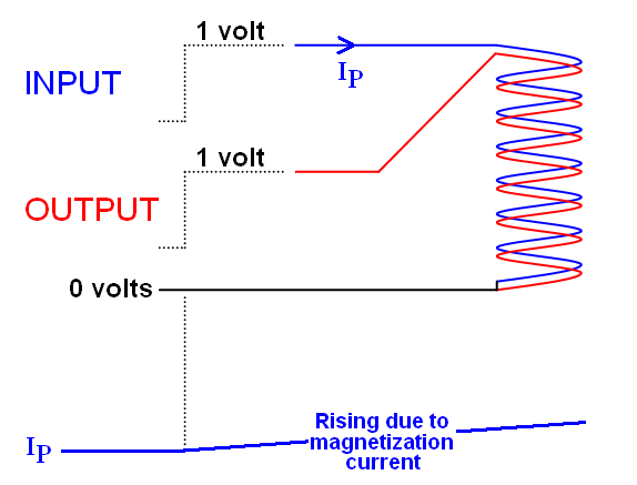
We should now consider what happens when the secondary winding is loaded with a 1 Ω resistor:

The instant that 1 volt is applied to the primary winding, the primary current becomes 1 amp. This is because of the induced 1 volt on the secondary winding that supplies 1 amp into its 1 Ω load: from ohm’s law and the conservation of energy.

We also see that as time passes, the primary current increases. It’s no different to when the secondary was unloaded, except that the primary current now has an offset of 1 amp due to the secondary current of 1 amp. Thus, the magnetization current ramps up at the same rate as previously seen, and that rate is still determined by the inductor formula:

V= Lᐧdidt

We say that the primary current (I_P) has two components; the secondary current (as referred to the primary) and the magnetization current. We use the words “referred to the primary” in case the turns ratio isn’t 1:1.

A bit about turns ratio

We have been previously considering a 1:1 transformer loaded with 1 Ω but, if the turns ratio were (say) 2:1, the secondary current “referred to the primary” would be 0.25 amps. This is because a 2:1 ratio will induce only 0.5 volts at the secondary, causing a secondary current of 0.5 amps. 

Because we know (for this idealized situation) that all the load power must be drawn from the primary power source, the primary referred load current must be 0.25 amps. This is because it matches the power of 0.25 watts dissipated in the secondary load resistor (0.5 volts x 0.5 amps).

Magnetization current remains the same

However, the magnetization current remains the same; it is wholly determined by the primary applied voltage and the primary inductance. It is a separate entity to the primary referred load current, and we should keep it as a separate entity when analyzing transformers. And there’s another reason...

If we look at the polarities of I_P and I_S, we see that I_P flows into the primary but I_S flows away from the secondary. Hence, if we ignore the magnetization current (for a moment) then, there is a current of 1 amp flowing into one winding and a current of 1 amp exiting another identical winding. 

Therefore, because each winding is identical, the two magnetic fluxes will cancel each other out.

And it doesn’t have to be a 1:1 transformer for this to happen because it’s the current multiplied by the number of turns that dictates the magnetic field intensity. Hence in a 10:1 transformer, if the secondary is drawing 10 amps, then that gets projected back to a primary load current of 1 amp, i.e., the “ampere-turns” on both windings are the same but have opposite polarity.

What this means is that the only source of magnetization is the magnetization current. The impact of this is that load currents do not contribute to core magnetism. At the start of this article, I posed this question:

Will the core saturate when the secondary load draws more current?

And now, it should be clear why this is no. I also posed this question:

Why won’t my transformer work at 1 Hz or DC?

The answer is that the primary is an inductor. As previously shown, if you apply a constant voltage to an inductor, the current will ramp up until the signal or power source can no longer sustain that rising current. This is why we use transformers with AC and, it is also why low-frequency transformers need much bigger core geometries than those that operate at higher frequencies. To prevent high magnetization current flow, we build low-frequency transformers with high inductance windings, and this necessitates many more turns of wire and much larger magnetic parts.

Leakage Inductance

Previously we have discussed an idealized 1:1 transformer, but we now need to think about something called leakage inductance. Not all the magnetic flux created by the primary “couples” to the secondary winding. This can be thought of as having a few primary winding turns being separated off to form an additional component in its own right. Those few turns will still produce a “localized” magnetic flux, but it won’t “couple” to the secondary. Those few turns also have inductance, and so, we can begin to think of a transformer as follows:

What we see above is an ideal transformer surrounded by the inductive components that make it less than ideal. L_M inside the purple box is the basic magnetization inductance that we have covered earlier; it creates the core’s magnetic flux. Two inductances have been added, L_P and L_S standing for primary leakage inductance and secondary leakage inductance.

If we ignore the magnetization inductance and consider the “ideal 1:1 transformer” as a perfect 1:1 power transformer, we can simply replace it with wires and redraw the schematic like this:

We can now see that L_P and L_S are in series between the primary voltage and any secondary load. A typical AC transformer might have 3% total leakage inductance compared to magnetization inductance, so if the total primary inductance is 1 henry, the leakage inductance will be around 30 mH.

An inductance of 30 mH at 50 or 60 Hz is about 10 Ω of reactance and not much of a concern. However, if we operate the transformer at 10 kHz, then the leakage reactance rises to 2000 Ω, and this will significantly degrade the transformer’s ability to transfer power to the secondary load. So, the third question posed was this:

Why isn’t my power transformer working at 10 kHz?

And the answer should now be clear. The final question posed at the start was this:

Why does my transformer get hot when there is no load?

And, to answer that, we need to consider power losses inside the transformer. 

Transformer Losses

A more realistic transformer equivalent circuit for our transformer is as follows:

Three resistors (R_P, R_S, and R_C) have been added to the schematic. R_P and R_S are the winding losses, i.e., the resistance of the copper wires used in the transformer. If you use more turns (to increase magnetization inductance), it increases the series resistance.

It’s a trade-off; we want to make magnetization inductance high to keep magnetization currents low, but by making L_M high, we need more winding turns, which means more series resistance losses. On the other hand, to keep series resistance (R_P, R_S) low, we would have to tolerate having higher levels of magnetization current. Unfortunately, this also comes at a cost because a higher magnetization current means higher core losses (represented by R_C). Core loss can cause a transformer to get quite warm because that power loss is driven by the applied primary voltage and not by load current (copper losses). Hence a transformer will still get hot when there is no load current.

If you want to know more, why not browse our product page for a more in-depth feature description or call an expert at Altium.