How Load Capacitance on a Transmission Line Affects Your Signals

If you ever read about transmission lines and integrated circuit datasheets, there is this seemingly mysterious quantity called load capacitance. This value depends on the geometry of the component lead connected to the transmission line, as well as the substrate material and distance to the reference plane on the integrated circuit die. When working with transmission lines, the load capacitance of a component has some important effects on signal behavior seen at the receiver, and it’s important to understand how you can affect the load capacitance in your PCB.
When you need to analyze signal behavior on a transmission line for a given load component, the load capacitance will affect S-parameters and the transmission line’s transfer function, so it needs to be included in high speed/high frequency signal analysis. In addition, the real input impedance at the load is determined by the load capacitance at sufficiently high frequencies. Here’s how you can better understand your load capacitance and determine how it affects signals in a transmission line on your PCB.
What is Load Capacitance?
The load capacitance on an integrated circuit is a parasitic element between the input lead and the nearest reference plane. In other words, the input pad connected to the component and the transmission line will see a shunt capacitance to the common ground reference (assuming the transmission line and the IC share the same ground plane).
This occurs because the pad connected to the transmission line is brought to some voltage as a signal reaches the receiver, but it is separated from the ground plane by the PCB substrate and the integrated circuit die. Note that the pin-package inductance has been omitted for the moment, which would sit as a series element between the transmission line and the pad. The parasitic capacitance between the pad/ground plane in parallel with the lead/die ground plane gives the total load capacitance. This is shown in the circuit diagram below:

For the above case of a differential channel, the applied termination is shown as a simple parallel resistor to simplify the picture involving differential signals. However, real termination circuits applied for a differential receiver can be more complex, as I've discussed in this article, and they are intended to preserve an offset while matching to the individual transmission lines in the channel, rather than matching to the differential impedance.
Termination
In the example above, the natural solution to addressing the inherent impedance mismatch is to apply termination. Consider shunt termination at the characteristic impedance (either integrated in the IC or applied with an external resistor). At low frequencies, the load impedance appears to be the terminated impedance. However, at high frequencies, the load impedance appears to be entirely due to the load capacitance. The takeaway here is: you’re only able to impedance match over a limited bandwidth due to the load capacitance.
Source-end Capacitance
One might naturally ask, what about the capacitance on the source side of the transmission line? Indeed, there is some source capacitance that determines the driver’s output impedance due to the presence of a pad. This is normally ignored when modeling because the signal that is sourced from the (driver + transmission line) system is only measured outside the driver. Therefore, we basically don’t worry about how the signal got there, just that we can measure what it is. We only need to worry about the input impedance of the (transmission line + load) system.
Transfer Function with Load Impedance
Whatever signal is launched into the transmission line will be affected by the load capacitance. This is then quantified with a transfer function. Intuitively, if you look at the diagram above, the capacitance acts like a shunt element to ground for high frequency components of the signal. Therefore a transmission line connected to a real IC acts like a low-pass filter, even before the signal reaches the load!
Intuition is nice, but how can we quantify this? Thankfully, you can examine the frequency response of the transmission line with a transfer function. This shows you, either in the Laplace domain or the frequency domain, how load impedance and transmission line’s characteristic impedance affect a signal in the frequency domain. You can then convert back to the time domain with a Fourier transform to compare the initial launch signal and the signal received at the load.
To do this, it’s by far easiest to use ABCD parameters for a transmission line. These are related to the S-parameters (insertion loss and return loss) for a single-ended line. The ABCD matrix for a single-ended line is defined in terms of the line’s characteristic impedance and has a similar meaning as S-parameters:

Now plug these values into the following general formula for the transfer function for a two-port network with defined source and load impedance (note the load impedance is shown above):

If we assume the source is matched to the transmission line, we have the following transfer function for the transmission line. I’ve written this in the Laplace domain for the moment:

Note that a very similar equation is presented in the literature on integrated circuit design for an electrically long line (i.e., longer than the critical length). This equation tells you exactly how the signal is affected by a transmission line’s impedance and the load capacitance. Note that, in general, the quantities in this equation are complex (including the propagation constant) and apply in the case where the line has any level of loss.
For this equation to be used for analysis, you need to include all the possible effects that can create distortion and loss in the system. These include:
- Dispersion and losses in the dielectric
- Copper roughness
- Skin effect losses as they relate to copper roughness
See this article to learn more about these sources of distortion and loss in your transmission lines and how to model them analytically.
Analyzing the Effects of Load Capacitance
Using a transfer function makes it very easy to analyze the effects of load capacitance on the transmission line and any propagating signals. This is best summarized in a graph. The plot below shows the transfer function magnitude and phase for a transmission line on FR4 (10 cm stripline, 0.48 mm plane-to-plane thickness/0.198 mm width, dispersionless, Dk = 4.4, loss tangent = 0.02) with 50 Ohm characteristic impedance with parallel termination. The low-pass behavior up to 1-10 GHz is clearly seen in the top plot.

From this plot we see that, as the load capacitance decreases, the low-pass rolloff does not occur until higher frequencies. We can get a few extra GHz of headroom just by using a component with smaller load capacitance. There is less distortion at midrange frequencies (below the first phase inversion) as the phase curve is flatter up to ~10 GHz. Both plots should illustrate the difficulty in impedance matching up to high frequencies in the signal bandwidth. Here, we haven’t even included copper roughness, fiber weave effects, or the skin effect in these calculations.
When working on high speed/high frequency designs, you can only control the parasitic load capacitance seen on a transmission line from the PCB side. The integrated circuit you choose will have a defined input capacitance that can’t be changed. However, there are 3 levers you can pull to control the total load capacitance seen by a transmission line:
- Surface layer laminate thickness. The PCB’s parasitic contribution to load capacitance is proportional to the layer thickness, so using a thinner laminate for the surface layer with an adjacent ground plane helps push rolloff to slightly higher frequencies.
- Laminate dielectric constant. The PCB’s contribution to total load capacitance is proportional to the laminate’s Dk value, so using a low-Dk laminate for the surface layer provides lower total load capacitance.
- Components. A component with a smaller lead size will tend to have smaller load capacitance. Keep this in mind when selecting components if you need to maintain signal integrity out to very high frequencies (~10’s of GHz).
Short Transmission Lines? Use a Circuit Simulator
When the line is electrically small, we don’t need to take a travelling wave approach and we can just use the circuit theory to describe a transmission line. This effectively forms a mismatched Pi network, which also exhibits low-pass behavior at high frequencies. The difference here is that resonances and transients can occur, just like you would see in a standard RLC circuit. To examine this type of system, you can use the circuit simulation tools in your schematic design software to understand signal behavior and design signal behavior to be critically damped.
Rise Time at the Load for Single-Ended, Non-Impedance Controlled Lines
On a bus like SPI, or with an equivalent signaling format over GPIOs with push-pull driving, the rise time on an electrically short bus will depend on the load capacitance. For example, if you look at the data for the rise time of a SPI driver, the rise time will depend on the load capacitance. This data may be available in the datasheets for the driving component, and the input pin capacitance should be available for your load component.
An example data table for XTAL signaling with the ADUC847 is shown below. The data table specifies a typical rise time of 9 ns for a load capacitance of 80 pF (marked in red boxes). You'll find similar examples for SPI/QSPI buses on other components, such as DSP ASICs, ADCs, MCUs, and a host of other digital/mixed-signal components.

In the above example component, there are logic interfaces that could be used with a range of possible digital signal rise times. In fact, if you look on page 91 of the datasheet for the ADUC847, you'll see the following recommendation from the manufacturer:
If the user plans to connect fast logic signals (rise/fall time < 5 ns) to any of the digital inputs of the ADuC845/ADuC847/ADuC848 add a series resistor to each relevant line to keep rise and fall times longer than 5 ns at the input pins of the device.
In case you weren't sure, it's important to realize that they are specifically telling you one of the main functions of a series termination resistor: to slow down the signal edge rate. This can be used to control damping on short transmission lines that have excessive underdamped oscillations (due to ground bounce and small load capacitance), as well as match the termination.
Which Circuit to Use for Simulation of a Short Bus?
To comprehensively account for load capacitance in a simulation with an I/O buffer, you need a few ingredients in your circuit:
- A simple buffer circuit that includes FET parasitics
- A load capacitance value
- A bypass capacitor value
- The total inductance of the line
- The capacitance of the line
- Inductance values for any vias connecting the power, ground and capacitor nets
An example circuit is shown below. This is the type of circuit that would be used to simulate ground bounce. It's important to understand that the load capacitance will contribute to the signal characteristics measured in this example, and it will determine any series termination you might need to apply on these short lines in order to match impedance and damp the signal simultaneously.

The above example would be implemented in your schematics and performed with SPICE. You don't need complex SPICE models for your driver component, you only need reasonably accurate SPICE models for the FETs used in the buffer circuit. The alternative is to specify the logic family used in your component in a 2D BEM/MoM simulation. An example can be found elsewhere on the blog.
Whenever you need to model transmission line behavior in pre-layout or simulate signal behavior post-layout, you can use the complete set of CAD tools in Altium Designer®. The integrated EM field solver in Altium Designer and signal integrity simulator lets you examine how load capacitance of standard logic families affects signal behavior on impedance controlled lines in your PCB. You’ll have a complete set of simulation features for your next board.
Altium Designer on Altium 365® delivers an unprecedented amount of integration to the electronics industry until now relegated to the world of software development, allowing designers to work from home and reach unprecedented levels of efficiency.
We have only scratched the surface of what is possible to do with Altium Designer on Altium 365. You can check the product page for a more in-depth feature description or one of the On-Demand Webinars.


About Author
Related Resources


Related Technical Documentation
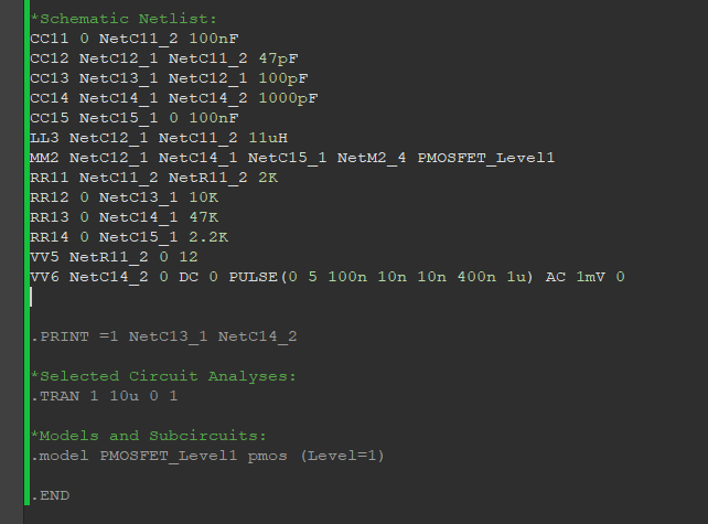

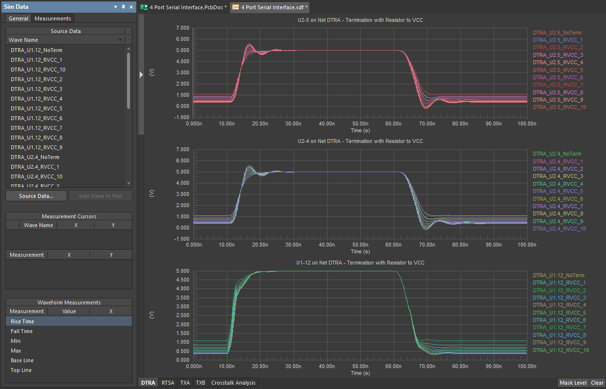


Table of Contents
- What is Load Capacitance?
- Termination
- Source-end Capacitance
- Transfer Function with Load Impedance
- Analyzing the Effects of Load Capacitance
- Short Transmission Lines? Use a Circuit Simulator
- Rise Time at the Load for Single-Ended, Non-Impedance Controlled Lines
- Which Circuit to Use for Simulation of a Short Bus?
Take advantage of the world's
most trusted PCB design system.
One interface. One data
model. Endless possibilities.
Effortlessly collaborate with
mechanical designers.
The world's most trusted
PCB design platform
Best in class interactive
routing
View License Options
Thank you, you are now subscribed to updates.