


How to Control Switching Signals with Terminations for Best Signal Quality


A transmission line is a pair of conductors used to deliver energy in the form of an electromagnetic field. Most of us are familiar with the wires that lead to our houses to deliver the power needed to operate our lights and appliances. In the context of PCB design, it is a signal in a signal layer on top of a plane or between two planes.
TRANSMISSION LINES AND TERMINATIONS
The purpose of this section is to explain what transmission lines are; what is moving on them, how they behave when switching signals are sent on them and how to control those switching signals with terminations for best signal quality. At the end of this section is a list of materials for further reading that may prove useful to the reader.
A key part of this section and the ones that follow is providing design rules that are valid along with the proof of their validity. It is the author’s belief that all design rules should be accompanied with their proofs as well as with what their limitations are, if any.
If you are looking for more applied information about how to apply these concepts in Altium Designer®, click below to watch the video and learn how to calculate impedance for a single and differential transmission line as just one example.

WHAT IS A TRANSMISSION LINE?
At its most basic a transmission is a pair of conductors used to deliver energy in the form of an electromagnetic field. Most of us are familiar with the wires that lead to our houses to deliver the power needed to operate our lights and appliances. In the context of PCB design, it is a signal in a signal layer on top of a plane or between two planes. Figure 1 illustrates the four types of transmission lines normally used in PCBs. As can be seen there are two main types; stripline and micro-stripline. The former a transmission line between two planes and the latter a transmission line on top of a plane. It is important to note that that the word ground was not used to describe the planes. The DC name of a plane is of no consequence when discussing electromagnetic fields.
Figure 1. Types of PCB Transmission Lines
Various combinations of these four transmission line configurations will be used to make up a PCB stackup. Controlling crosstalk as signals run side by side in a signal layer or one over the top of another in adjacent signal layers will be covered in the next block. Also, calculating impedance will be covered in the following block.
Working through a transmission line through your various implements can be a bear. Mind you, with the right PCB design software, you ought be able to control impedance and crosstalk with smart design rules checking as well as manage PCB layer stackups with ease and grace. Altium Designer has kept these in mind when designing its user-friendly design environment.
Altium Designer’s Unified Design Environment
WHAT IS MOVING IN A TRANSMISSION LINE?
In order to properly manage a transmission line it is important to know what is moving on that transmission line. In beginning electronics we are taught about voltage and current with current flow identified as the signal. Unfortunately, this is too simplistic a view of how signaling happens and if the focus is on current flow only, the quality of signals may be compromised.
Most of us know that electronic signals move at or near the speed of light which is at or near 186,000 miles or 300,000 kilometers per second in a vacuum. Current flow, which is the movement of electrons in a copper conductor moves at the rate of about 1375 miles per hour or 2200 kilometers per hour. So, the signal can’t be current flow. It is the electromagnetic field. Figure 2 illustrates what the electromagnetic field looks like around a stripline transmission line. The line is coming out of the page travelling between two planes and is an end on view.
Figure 2. Electromagnetic Field Around a Stripline Transmission Line
Notice that there are two field types in the drawing, electric field lines that extend between the transmission line and the two planes and magnetic field lines that surround the transmission line. It is the magnetic field that displaces electrons in the transmission line which we can measure with an ammeter and which we call current flow. An equal and opposite current flows in the two planes that we often call return current. How this return current is split between the two planes is a function of how close each plane is to the transmission line.
Knowing how to create and manage electromagnetic fields is the key to succeeding in high speed electronics.
CREATING AND MANAGING ELECTROMAGNETIC FIELDS
Every electronic signal is intended to deliver a voltage waveform to a receiver. To do this, energy in the form of an electromagnetic field is created and sent on a transmission line to the receiver. Figure 3 is a typical signal path with a driver, a receiver and a transmission line connecting them.
To deliver the highest quality voltage waveform to the receiver, it is important that the signal not be degraded as it travels from source to receiver. The most common form of degradation is reflections of part of the signal (energy) at impedance mismatches. Ideally, Zout = Zo = Zload resulting in no reflections. Signal integrity engineering strives to meet this requirement by designing PCB stack-ups to hit a target impedance and by adding terminations to reduce mismatches.
Figure 3. Typical Signal Path With Source, Load and Transmission Line
Terminations
Once the electromagnetic energy sent down a transmission line has delivered the voltage waveform to the receiver, it must be removed from the system or it will reflect around causing unwanted transients that may result in false triggering of loads along the line or destroying an input if the reflections are too large. The purpose of terminations is to remove this energy once the voltage waveform has been delivered.
There are two types of terminations. These are series and parallel. Figure 4 illustrates types of terminations that might be used and how these terminations are connected to a transmission line. The series terminations are connected in the net at the output of the driver. How this termination removes the EM energy from the transmission line is explained in the next section. Parallel terminations are attached at the driver end of a transmission line to remove the EM energy as it arrives at the receiver.
Figure 4. Types of Terminations
In figure 4 notice that there are four terminations placed at the receiver end of the transmission line near the receiver. These are various way parallel terminations have been implemented. The merits of each will be discussed later. There is only one termination located near the driver. This is a series termination. How it works to control reflections is addressed in the next section.
The four options for parallel terminations are: AC, diode, Thevenin and single resistor to a terminating voltage.
AC terminations have their origin in the days of TTL when rise time got fast enough to require a parallel termination at the receiver. TTL could not support the DC loading of a 50-ohm termination, so a capacitor was used to connect the termination to the transmission line allowing it to absorb the energy in the fast switching edge while remaining disconnected during steady state conditions. This worked as long as the ratio of rise time to clock rate was very large. As clock speed increased the degradation shown in Figure 5 resulted degrading the signal such that is was not useable. The red waveform is the signal leaving the driver and the orange waveform is the signal arriving at the receiver. Clearly, this is an unsatisfactory way to parallel terminate a transmission line and should never be used.
Figure 4. AC Terminated Clock at 66 MHz
Diode terminations came into existence when overshoot, reflections that rise above Vdd or extend below ground, exceeded the input voltage rating of the receivers. As will be shown, this problem can be avoided by using simple parallel or series terminations. Diode termination is a very expensive way to control overshoot and should never be used.
There is one exception to this. The PCI bus requires series terminations in the outputs of all drivers. Engineers who designed add-in cards for PCs who did not understand this omitted the series terminating resistors to save cost. When these cards were plugged into a PC motherboard there was often a failure from overshoot. The consortium that maintains the PCI bus standard could not prevent this from happening and put a requirement in the spec that all inputs must have diodes on their inputs to be PCI compliant solving the problem.
Resistive parallel terminations are the simplest way to terminate a transmission line. Figure 5 is an illustration of a GTL bus with a parallel termination. Notice that the terminating resistor connects to a terminator voltage, usually labelled Vtt which is a separate power supply from Vdd. This means that a system using parallel terminations requires two power supplies capable of supplying very fast switching transients. When a system has many transmission lines that must be parallel terminated this extra cost is worth it. When there are only a few lines that need to be parallel terminated, such as the clock lines in some DDR configurations, this extra cost can be a burden. This is when a Thevenin termination is useful.
Figure 5. Parallel Terminated GTL Transmission Line
Thevenin parallel terminations are a method of creating the equivalent of the Vtt and Rt needed to parallel terminate a transmission line without requiring a separate power supply for Vtt. Figure 6 is the method for calculating the resistor values for a Thevenin terminating network along with a sample calculation.
Figure 6. Method for Calculating Thevenin Terminating Resistor Values
How Series Termination Works
Series terminated transmission lines are the primary method of connecting CMOS logic devices. Understanding how these transmission lines work is vital to making sure signals are properly delivered to each receiver. How all of this works is not intuitive and baffles some of us until it is explained. This short write up is intended to clear up some of the confusion.
Figure 7 is a typical 5V CMOS driver with a 50-ohm transmission line connected to a CMOS receiver that is passive meaning that it simply responds to the voltage waveform presented at its input. (For purposes of this explanation, CMOS receivers look like very small capacitors that can be considered to be open circuits.) In this example, the line is 12” or about 30 cm long. In a PCB, energy travels at approximately six inches per nanosecond, so this line is about two nanoseconds long.
Figure 7. A Typical Series Terminated 5V CMOS Circuit
Figure 8. An Equivalent Circuit for the Transmission Line in Figure 7
Notice that there is capacitance, resistance and inductance distributed along the length of the transmission line. These elements are called parasitics and determine the behavior of a transmission line with the ratio of inductance per unit length to capacitance per unit length determining the impedance of the line as shown in Equation 2.
Lo is inductance per unit length and Co is capacitance per unit length. These two variables are determined for a particular type of transmission line using a tool such as a 2D field solver. There are many field solvers available as parts of signal integrity tools.
In almost all cases, the value of R is so small compared to the L and C that it can be ignored. Until frequencies involved go above a GHz, this is a reasonable assumption.
Equation 2. Impedance as a Function of Distributed Capacitance and Inductance
When the driver in Figure 7 wishes to move the logic level on the transmission line from a logic 0 to a logic 1 it must charge up the distributed parasitic capacitance of the transmission line. This is the primary power consumed by CMOS logic circuits. When the same driver wishes to move the logic level from a logic 1 to a logic 0 it must remove that charge.
Tip: When a signal is sent along a wire or transmission line it is energy in the form of an electromagnetic field. This energy will travel along the path and be reflected at the ends of the path forever unless it is absorbed by a terminating resistor or is slowly lost in the resistance of the conductor. If the ends of the path are open circuits, the reflected energy will be the same polarity as the incident energy. If the ends of the path are short circuits, the reflected energy will be inverted.
How Charge Is Put on a Logic Line to Move It from a Zero to a One
Figure 9 is the equivalent circuit of Figure 7 at the moment that the driver starts to move the logic line from a zero to a one. Notice that a voltage divider has been formed by the combination of the driver output impedance and the series termination in the upper part and the impedance of the transmission line in the lower part. When the series termination has been properly chosen the combination of Zout and Zst will be the same as Zo. In this example, both will be 50 ohms and so the voltage at the input to the transmission line will be V/2.
Figure 9. Equivalent Circuit of Figure 7 When a Transition from a Zero to a One Begins
Figure 10 shows the voltage waveforms at the input to the transmission line and at the input to the receiver as time goes by. The red waveform is the input to the transmission line and the orange waveform is the input to the receiver at the end of the transmission line. Notice that the voltage level immediately after the transition from zero to one is only half of Vdd or half size. This is because of the voltage divider shown in Figure 9. This voltage level is often referred to as the “bench” voltage.
What has been launched into the transmission line is energy in the form of an electromagnetic field (EM) the voltage component of which is V/2. This energy is charging the parasitic capacitance of the transmission line to a voltage level of V/2 as the field travels out the transmission line.
After two nanoseconds (the electrical length of the transmission line) the line has been fully charged to V/2 and the electromagnetic field encounters an open circuit at the receiver. When such a field encounters an open circuit none of the energy in the field is absorbed and it is reflected back at the same magnitude it had when it was outbound.
At the moment of total reflection, the voltage level on the end of the line is V/2. Since the voltage magnitude of the electromagnetic field is V/2 after total reflection the amplitude will be V. Notice that the orange waveform has an amplitude of V as soon as the EM field arrives at the end of the line. On the return trip, the parasitic capacitance of the transmission line is charged all the way up to V. Once the electromagnetic field returns to the driver it encounters the equivalent circuit shown in Figure 11.
Figure 10. Voltage Waveforms at The Two Ends of The Transmission Line in Figure 7.
Figure 11. Equivalent Circuit of the Driver in Figure 7 Seen by the Reflected Electromagnetic Field
Since the sum of Zout and Zst is 50 ohms, and the voltage source is a short circuit. Together they constitute a parallel termination that has the same value as the line impedance. As a result, all of the energy in the electromagnetic field is absorbed and the voltage level on the transmission line stabilizes at 5 volts which is an ideal logic 1 for this circuit.
Switching from a Logic 1 to a Logic 0
When the circuit in Figure 8 switches from a logic 1 to a logic 0 the driver has the task of removing the charge on the line capacitance that was put there in order to move it from a logic 0 to a logic 1. To do this the driver level moves internally from 5V to 0V. As with the transition from a logic 0 to a logic 1 the equivalent circuit is like that shown in Figure 9, but, now, the line is at 5V and the output impedance and series terminating resistor are connected to 0V. The voltage divider is at work as it was before.
As a result, the line voltage is moved to V/2 and charge is removed from the line capacitance to this level as the energy moves down the line. (The voltage level of this transitions is –V/2.) When the EM field arrives at the end of the transmission line two nanoseconds later it encounters an open circuit and is reflected back down the line. The result after the reflection takes place is the line is now at 0V. Two nanoseconds later the EM field arrives back at the driver and encounters the circuit shown in Figure 5 and is absorbed. The resulting waveform is shown in Figure 12.
Figure 12. Voltage Waveforms at the Two Ends of the Transmission Line after Switching From 1 to 0
Notice that the voltage waveform at the receiver (orange) is a proper square wave logic signal which is the goal of this signal path. This signaling method is known as “reflected wave” switching because the correct logic level is created by the reflected wave as it makes its round trip along the transmission line. This is the lowest power consumption method of high speed logic signaling because current is only being drawn from the power system while the line is being charged. Once the line has been fully charged to a logic 1 the current draw goes to zero.
This is the switching method that is employed with the PCI bus that is incorporated into most personal computers.
Also, notice that the voltage waveform at the driver output is at an indeterminate logic state for a time that is the round-trip delay along the transmission line each time switching takes place. If loads are placed along the length of the transmission line, as is done with the PCI bus, they do not experience a “data good” condition until the reflected wave passes by them on the return trip. Therefore, clocking of data at these inputs must be delayed until data is good at all inputs. This is how data is clocked on the PCI bus and other bus protocols that rely on reflected wave switching.
Impedance Editor within Altium Designer’s Rules and Constraints Editor
What Happens When the Driver Impedance Does Not Match the Line Impedance?
The circuit shown in Figure 13 is the same as that shown in Figure 7 except that the series termination has not been inserted in series with the output.
Figure 13. An Unterminated 5V CMOS Transmission Line
Figure 14 shows the switching waveform for the transition from a logic 0 to a logic 1. Notice that the bench voltage is much higher than V/2. In fact, it is 2V/3 or 2/3 of the total of 5 volts or 3.33V. Why is this? If you refer to the voltage divider in Figure 3 in this example the upper resistance is 25 ohms or Zout of the driver and the lower resistance or impedance is 50 ohms producing the 2/3 voltage level.
The EM field is charging the line capacitance to this value as before. When the EM field arrives at the receiver two nanoseconds after being generated it is reflected back, doubling the voltage to 6.66V. As before, the EM field charges the line capacitance up to 6.66V. After another two nanoseconds the EM field arrives back at the driver and encounters a termination like that shown in Figure 5. However, the parallel termination is not 50 ohms. Instead it is 25 ohms. Two things will happen. First, the voltage divider this time is 50 ohms on top and 25 ohms on the bottom as shown in Figure 15 with the series terminator value being zero ohms, so the voltage is divided down. Second, not all of the energy will be absorbed.
When an EM field encounters a parallel termination that is lower in value than the TL, the reflected energy will be the opposite polarity of the incident waveform. This cannot be seen at the driver. Two nanoseconds later the energy arrives at the receiver and, as can be seen, it is inverted or is negative going.
As before, the amount of energy will double the voltage level at the receiver and travel back toward the driver. When it arrives at the driver some of it is absorbed and the rest is reflected inverted. This goes on until such time as all of the energy has been absorbed in the driver output impedance and the logic level settles out at 5V. This can be seen in Figure 16.
Figure 14. Switching Waveform for an Unterminated CMOS Transmission Line
Figure 15. Equivalent Circuit of Figure 13, Zst = 0
Figure 16. Switching Waveform for an Unterminated CMOS Transmission Line
There are two problems with the waveform in Figure 16. First, the voltage goes 1.66 volts above Vdd. This excess voltage can cause logic failures or damage the receiver. Second, after the signal arrives back at the drive and is inverted, it causes the logic 1 at the receiver to drop to below 4 volts. This diminishes the logic one to a level that could result in a logic failure. Neither of these is good. That is why a series termination is added to a circuit like this.
Figure 17 shows the waveform when the signal switches to a logic zero. As you can see, the same level violations happen in this logic state.
Scale is 1 Volt per division with the bottom line at -1 V and the top at 8 V
Figure 17. Another Switching Waveform for an Unterminated CMOS Transmission Line
Overshoot and Undershoot
The terms overshoot and undershoot are used to describe unwanted excursions of signal waveforms due to reflections caused by impedance changes. Figure 18 depicts a 50-ohm parallel terminated transmission line. with three different values of terminating resistor. The waveforms shown are measured at the driver output. When a transmission line is perfectly terminated in its characteristic impedance, in this case 50 ohms, all of the energy is absorbed by the terminator as it arrives at the receiver and no energy reflects back toward the driver. This is shown by the center waveform in Figure 18.
Figure 18. Parallel Terminated Transmission Line
When the terminator value was changed to 70 ohms, the line was no longer perfectly terminated and some of the energy reflected back to the driver. Equation 3 is often called the reflection equation. It is used to calculate the amount of reflection that will occur at an impedance mismatch. In the equation, Zl is the upstream impedance and Zo is the downstream impedance. In this case, the upstream impedance is the line impedance, 50-ohms, and the downstream impedance is the termination resistor. With the terminating resistor at 70 ohms the equation predicts that there will be a reflection of 16% of the incident voltage and the polarity will be positive, adding to the incident voltage as can be seen in Figure18, causing overshoot.
When the terminator value is changed to 30 ohms, again, the line is no longer perfectly terminated and some of the energy reflects back to the driver. Using Equation 3, the reflected value is 25%, but the value is negative, taking away from the incident value. This is called undershoot.
Equation 3. The Reflection Equation
When logic voltages were in the range of 5 Volts, the overshoot often got so large that it caused logic failures or even circuit damage. For this reason, the emphasis has always been on avoiding excessive overshoot. That is the reason for diodes on inputs. As logic levels have continued to drop, the probability of a failure from this have lessened. At the same time logic levels have dropped, the noise margin has also lessened making logic failures from coupled noise a big issue. As a result, more focus is on avoiding undershoot with most current logic families.
Determining Terminating Resistor Values
As noted earlier there are two types of terminations: series and parallel. The value for a parallel termination is the impedance of the transmission line being terminated. Determining series terminating resistor values is not so straight forward. The series terminating resistor is intended to add up to the transmission line impedance when combined with the output impedance of the driver. In other words, Zst = Zo – Zout. Where is the output impedance of the driver obtained? It would be nice if this information was printed as part of the component data sheet. Unfortunately, this is rarely the case. In order to find Zout, it is necessary to get the IBIS or SPICE model of the output driver and calculate it from the VI curve. Most of the SI modeling tools will do this calculation and display the output impedance. Some will even do the math and recommend a series resistor value.
This is where having a live-updating and easily accessible component library with access to supplier information and easy to update part models can be particularly helpful. Thankfully, as part of Altium Designer you have access to a wide array of component libraries and real-time updating supplier information easily accessible from any avenue of your production team.
Location of Terminations
The question often arises about how close a termination needs to be placed to the end of a transmission line in order for it to do its job properly. It would be good to place these resistors on the PCB surface in such a way that they don’t make layout or assembly unnecessarily difficult.
Locating parallel resistors is relatively easy. Anywhere after the signal has been delivered to the device input is fine as the voltage waveform has been delivered and the energy simply needs to be removed. Knowing this, place the parallel terminations after the last load on the transmission line out of the way. No need to cram them under BGA pin field, so that routing the PCB and assembly is eased.
Locating series terminations requires a little more analysis. Since the series terminating resistor is intended to sum up with the output impedance of the driver, it needs to be close enough meaning that the trace connecting the two, is short enough that it does not function as a transmission line isolating one resistance from the other. The only way to arrive at an acceptable length for the connection is to use a simulator to see how long this connection can be and still have an acceptable waveform at the receiver. It will turn out that the allowable length is a direct function of the rise time of the driver. The faster the rise time, the shorter the allowable connection.
Stubs
A stub is a branch off the main transmission line. Under certain conditions a stub can adversely affect a signal. When a stub is long enough, it appears to momentarily short out the signal. Figure 20 depicts a transmission line one quarter wavelength long at some frequency F.
Figure 19. Transmission Line with Stub
In Figure 20, a sine wave is shown launched at the input to the transmission line. A quarter wavelength later, or 90 degrees later, it arrives at the open end of the transmission line which is an open circuit. Since the end is open, all of the energy is reflected back without being inverted. A quarter wavelength later it arrives back at the input exactly 180 degrees out of phase with the input signal, canceling it. The effect is a short circuit at the frequency F.
RF engineers use quarter wave stubs as band stop filters in some parts of radios where there is a single frequency that is causing interference. Unfortunately, there are few places in logic where eliminating a single frequency is called for. Instead, stubs cause waveform reversals such as the blue waveform shown in Figure 21. This waveform reversal is on a clock resulting in double clocking.
Figure 20. Waveform on Quarter Wave Transmission Line
Figure 21. Waveforms on a Clock Line Showing Results of a Stub
The only method that is reliable for deciding if a stub is short enough to avoid causing the problem shown in Figure 21 is to simulate the proposed topology in a tool such as Hyperlynx and see if the waveform degradation is acceptable. Because the rise times of many current ICs is so fast (often less that 100 pSec) the length of the trace from the ball on a BGA to the actual contact on the die itself can be long enough to cause a problem. This length must be included in the simulation.
Vias
Via is a term used to describe the plated through hole used to connect the signal pin of an IC to a trace on an inner layer of a PCB or to a trace on the opposite side of the PCB. These vias are plated through holes that have both capacitance and inductance. The inductance of the via will be approximately 35 picohenries per mil of length (1.4 nanohenries per mm). Whether or not this inductance will be a problem depends on how the via is used.
If the via is used to connect a bypass capacitor to a plane or a component power lead to a plane, this inductance may be a problem with very fast rise time signals or degrading performance of bypass capacitors.
Layer Stackup management made easy
Most vias are created with drills of 12 mils (.3 mm) or smaller. A via created with a 12-mil drill in a PCB 100 mils (2.5 mm) thick will average about 0.3 pF. Whether or not this added capacitance will cause a signal integrity problem is best answered using a good simulator. From experience, the author has observed that for data rates up to about 3 Gb/S, the degradation from a vias is acceptable.
Strong layer stackup management within your PCB design software and an easy-to-transition between 3D model viewer will help to incorporate Vias and keep track of them within your designs. Don’t let vias and microvia management cause your designs to stumble when they’re so close to the finish line.
Vias in Altium Designer’s 3D model viewer
Right Angle Bends
The effect of right angle bends in signal traces have worried over for as long as PCBs have been manufactured. Some of the effects that have been mentioned are:
- Right angle bends cause EMI.
- Right angle bends cause signal integrity problems.
- Right angle bends cause acid traps during PCB fabrication.
Sample of angles of trace routing
In some cases, a great deal of effort has been expended to make sure right-angle bends are eliminated. There have even been entire CAD systems scrapped because they could not be prevented from placing right angle bends in traces. A fair question would be “Are right angle bends a problem with logic circuits?” Item 1 at the end of this section describes a test PCB constructed to measure the effects of right angle bends. This PCB was designed with right angle bends, acute angle bends and obtuse angle bends to see what they look like from the point of view of the three concerns listed above. Testing was done in the EMI laboratory at the University of Missouri, Rolla.
The results of this testing is that none of the things right angle bends are supposed to cause actually happen. A fair question might be how did these ideas come to exist? The most likely way was the observation that RF engineers round off all corners. This is done because corona discharge occurs at sharp corners at high RF power levels.
The curious thing is that the fact that right angle bends do not cause trouble has been known for at least 40 years and demonstrated with tests and published papers. Yet the myths continue to be passed on from engineer to engineer.
Keeping in mind signal integrity principles as well as transmission lines and termination principles is a task in and among itself. With the right design software, a lot of the work can be done for you though from the onset of programming the right design rules and having proper signal integrity analysis tools. Make sure you’re using the design software which will be doing the work for you.
With advanced design tools, a unified environment, and industry-standard rule verification included, in Altium Designer you can seamlessly build anything you can imagine. Click on the free trial and try it out.
Click on the free trial to try it for yourself or watch the OnTrack Podcast episode with guest Lee Ritchey below.
Sign up and try Altium Designer 19 today.
About Author
Related Resources
Table of Contents
Design to Release, Without the Friction
- Keep reviews tied to the right version
- Reduce handoff confusion and rework
- Spot sourcing and release risk earlier
- Work solo, share when needed
Get Started
Thank you, you are now subscribed to updates.


