


Channel Operating Margin Isn’t So Bad

At a Glance
What is Channel Operating Margin? What does Channel Operating Margin metric actually means. This blog will trace the evolution of COM back to its roots and put meaning to the infamous COM metric.


What is a COM anyway?
Channel Operating Margin, or COM, is a summative metric for characterizing channel signal integrity, either from simulation or measurement. Due to the requirement for testing multiple equalization and FEC settings, it is more often used as in simulation for predicting channel signal integrity in the presence of noise in a channel. Thought of another way, COM is a type of signal-to-noise ratio (SNR) metric, but it includes equalization settings lumped into the signal and noise calculation, giving a prediction for best-case signal integrity.
COM isn’t well understood. Since it isn’t well understood, many people doubt it really means anything. After all, how can channel quality be represented by just one number in decibels? It turns out, COM is actually the latest evolutionary step in a long progression of channel validation techniques using eye patterns. This blog will trace the evolution of COM back to its roots and put meaning to the infamous COM metric.
The First Channel Operating Margin: Eye Patterns
Let’s start with eye patterns. Eye patterns are a way to look at a long stream of serial data. Back before Keysight ADS and PyBERT, an eye pattern was measured with a digital sampling oscilloscope or a real-time scope. In the eye pattern window, the y-axis units are voltage and the x-axis units are time spanning two unit intervals. A unit interval, or UI, is the amount of time for one bit to pass. Thus within two UI of time, you can center one bit data on the screen with half of a bit of margin on either side. However instead of viewing just one bit, all of the bits are overlapped, one at a time, until the entire stream of serial data is on the screen. The signal quality is quantified by the size of the hole in the middle. If the eye pattern looks really good, you might hear an engineer say, “You can drive a truck through that eye!” The most common ways of quantifying the opening are width, height, or area. The crossing of the eye at the DC point is the jitter, and the jitter is typically measured statistically with a histogram.
Figure 1. Example of a serial bit stream.
Early channel specifications, and in some cases passive component specifications, used something called an eye mask for the pass/fail criteria. An eye mask is usually a diamond-shaped area defined by an eye width and height. A passing eye has only so many detected samples or hits, inside the eye mask. The patterns of ones and zeros are dictated by the standard and are usually pseudo-random bit sequence or PRBS pattern. You can basically bank the patterns into two categories: before 10 Gb/s and after 10 Gb/s. Before 10 Gb/s 8b10b encoding was used in most systems and PRBS 7 was the appropriate pattern. When 10 Gb/s was introduced by the IEEE in 802.3ba, the encoding switched to a 64b66b scrambler and PRBS 31 took over. Even today at 112 Gb/s, PRBS 31, or QPRBS 31, is still the standard pattern most use.
For 224G per-lane COM, the pattern to keep in mind is PRBS13Q. One of the 2024 DesignCon papers specifically compares the proposed OIF CEI-224G/IEEE 802.3dj COM methods based on a PRBS13Q pattern and demonstrated COM-style calculations. However, not every 224G lab demo or interoperability setup uses the same PRBS pattern. For example, OIF’s 224G LR/MR and linear demos used PRBS13Q, while an OIF 224G-VSR demo used PRBS31Q.
For 448G per lane, there is not a single finalized COM PRBS because 448G is still being defined. As of 2026, OIF’s current 448G work shows the modulation is still effectively TBD, and public OIF material describes 448G demos and framework work spanning PAM4, PAM6, and PAM8, with test methodologies still under development.
Statistically Speaking
Chronologically after measured eye patterns, StatEye is the next method of qualifying passive channels, and it was heavily used by the OIF. The idea behind StatEye is explained in detail here. In brief, StatEye predicts eye patterns using a pulse response of a system. A pulse response is the time-domain response of a system excited with a one-UI square pulse, and the system is a passive channel including equalization. The equalization technologies available in StatEye are FFE, CTLE, and DFE. The transfer function of a system is gathered from S-parameters. Since channel S-parameters can be simulated, StatEye is an efficient way to try many channels and equalization settings to see what works. All the while, the eye mask is the pass/fail criteria using the statistically predicted eye opening.
Somewhere between StatEye and COM, peak distortion analysis (PDA) became somewhat common. The method is well documented by Heck and Hall in Advanced Signal Integrity for High Speed Digital Designs. In summary, it uses the same pulse response as StatEye, but it’s output is simply the so-called worst case eye opening. PDA doesn’t make up any data, and that is the reason I personally like it. I’ve implemented it myself and found PDA predicts worst case eye patterns with high confidence. However, PDA and StatEye do not include the impact of the transmitter and receiver in the channel, and you need to find the best equalization setting manually.
Figure 2: Example of an Eye Pattern in blue and PDA in dashed black.
Enter COM
COM was developed as part of IEEE 802.3bj, 100GBASE Ethernet, and added the IC imperfections to the simulated channel. It is easier to use and more widely adopted than StatEye, and is the defacto channel quality prediction tool today. As I already mentioned, COM builds from StatEye and adds several new noise sources. Specifically, the noise sources are loss from the IC, IC package reflections, IC related jitter, and a lumped Gaussian noise source for all other stuff happening in the IC, like crosstalk. The implementation of COM is found in IEEE 802.3 Annex 93A.
Most of the math behind COM is simplified by the standard body as much as possible. For instance, S-parameter concatenation is reduced to algebra instead of conversions From S-parameters to ABCD-parameters or T-parameters and matrix multiplication. The most difficult equation is calculating the probability density function (PDF) of ISI related noise, but after a few tries it’s really not too bad. There are some omissions that are considered implementation specific, such as how to ensure 32 sample points within every UI of data, but these details can be found within the open-source code provided freely by the IEEE.
COM finds the best case scenario for a given channel using a set of possible equalization settings. This is accomplished by sweeping all equalization settings and calculating something called the Figure of Merit (FOM). The equalization setting that produces the best FOM is used for the remainder of the calculations. Once the PDFs of all noise sources are calculated, the noise at a detected error rate (DER) is identified. The DER is the desired bit error rate (BER) for the system, and is determined by what Forward Error Corrections (FEC) technique, if any, is being considered. The available signal is determined by the pulse response voltage at a specific sampling point. The available signal is divided by the noise at the detected error rate (SNR), and this number is converted into decibels. Voilla! COM! See, it actually does have meaning.
Mathematically, the formula for calculating COM is given in the following equation:
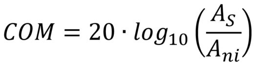
Where As = signal level with best-case equalization settings (highest FOM), and Ani = SNR at the targeted DER value.
The settings used for COM are determined by the available IC technology. The level of IC technology is agreed upon by industry leaders such as Intel, Broadcom, Mellanox, Fujitsu, and many others. In other words, an IC using technology implemented in COM should be able to function in working channels as predicted by COM. Obviously, this is very powerful since the standard has now (finally) put some of the channel ownership onto the IC vendors.
Even though it sounds like COM is this utopia of channel prediction, it does have limitations. Since it is one set of settings for all systems being considered by the standard, it does not predict the performance of any one IC by itself. To get measurement correlation, you need to adjust the COM settings for each individual IC. Further, COM neglects any noise contribution from skew. Fortunately, a DesignCon paper by Jason Chan addresses this deficiency, and I hope to see updated COM scripts utilizing his ideas in the future.
Conclusion
To sum it up, COM is not so bad. It is a very logical next step in the evolution of channel analysis, and it makes channel evaluation relatively easy. I’m very grateful that the authors of COM were kind enough to freely release and support the MATLAB code. I hope to see COM implemented and improved by other signal integrity engineers in the future. Who knows, maybe we’ll see a Python or Octave implementation someday.
Translate channel analysis like COM into clearer design decisions you can trust. Altium Develop helps engineers keep signal‑integrity intent, design changes, and reviews tied to the active design so analysis results inform layout and release without added workflow friction. Get started with Altium Develop today →
All figures were created with GNU Octave.
About Author
Related Resources
Related Technical Documentation
Table of Contents
Design to Release, Without the Friction
- Keep reviews tied to the right version
- Reduce handoff confusion and rework
- Spot sourcing and release risk earlier
- Work solo, share when needed
Get Started
Thank you, you are now subscribed to updates.

