Where Does the -10 dB S11 Limit Come From?

S11 plots, or equivalently return loss plots, show the amount of signal loss due to reflection as it enters an interconnect and encounters impedance discontinuities on its path to a load. There is a practical limit you often enforce on return loss plots, beyond which we consider the reflections to be excessive. This maximum acceptable value in an S11 plot is typically taken as −10 dB, and it has become something of a de facto standard used in signal integrity.

In reality, this value comes from a very specific situation involving RF design, and it has been brought over to digital design without much worry as to its relation to characteristic impedance and/or input impedance. If you do some math on the power reflection coefficient and the voltage reflection coefficient, and then relate this to the typical 10% tolerances specified for high-speed interfaces, you will find that there is a one-to-one relationship between this −10 dB limit and impedance tolerance. We will explore how these tolerances and reflection limits correspond in this article.

What is the −10 dB S11 Limit?

When examining S11 plots for an interconnect, the goal is to determine when reflections are excessive and whether design changes are needed. The −10 dB limit is a de facto limit above which we often consider reflections to be excessive within a particular frequency range.

An example in a 10 GbE differential pair is given below. The image shows the selected link in a PCB and the S-parameters from the input board-to-board connector to the output SFP+ connector pins, which will connect to an optical transceiver. The SDD11 graph is shown in the upper right, and the green line is at −10 dB on the y-axis.

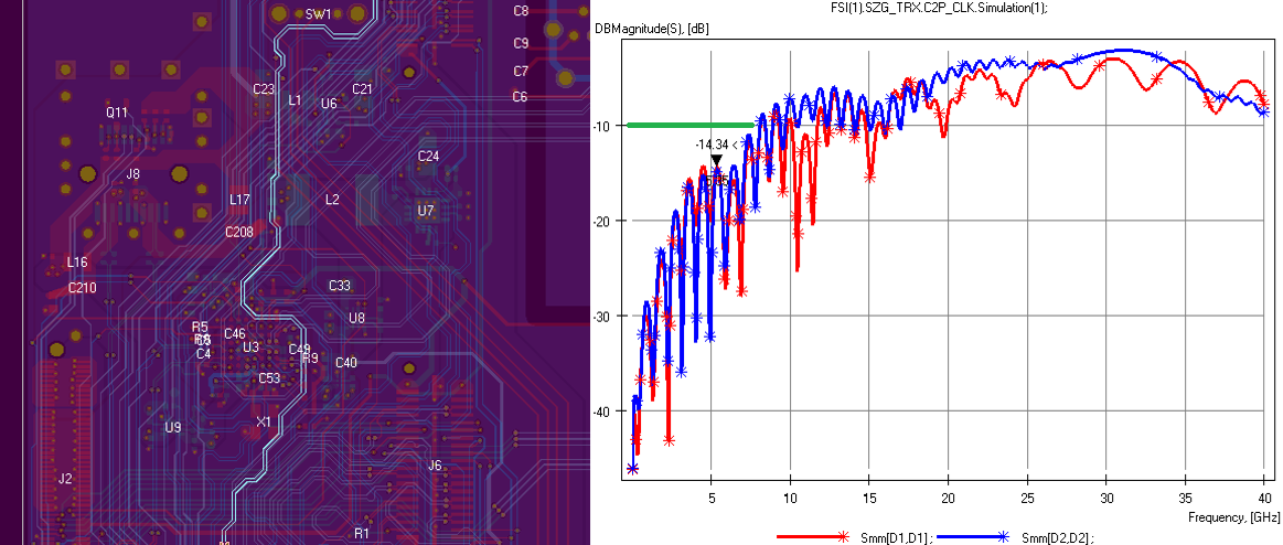
The SDD11 graph tells us that below approximately 15 GHz, the impedance is matched very closely to the target of 100 ohms. Above this, the impedance match very quickly diverges, and the reflections become rather strong. Together, the SDD11 and SDD21 graphs indicate that the impedance is reasonably closely matched and loss is low enough within the bandwidth required for the interface. This means that the link has a good chance of working as long as other conditions can be met. Note that it does not automatically mean the link works perfectly, but it is a good first indicator that impedance is sufficiently matched within the bandwidth required by the interface.

Power Reflection Coefficient Versus Voltage Reflection Coefficient

It is often said that an S11 plot or a return loss plot is the reflection coefficient in decibels. Although technically correct, we have to understand which type of reflection coefficient we are referring to. There are two types: power reflection and voltage reflection.

• Power reflection refers to the reflection of the voltage and current waves, which are then multiplied together to give the total power.
• Voltage reflection refers specifically to reflection of the amplitude of the voltage wave of a signal.

The reason we have these two definitions is simple: in reactive interconnects or circuits, the voltage and current are not always in phase at all frequencies. In digital designs, and specifically in transmission lines, the reactive component tends to be very small, and therefore the current is almost always in phase with the voltage, so we just use the voltage reflection coefficient. We also use the voltage reflection coefficient because noise margins and logic thresholds are specified in terms of voltage values, not power values. However, RF designers may like to use power reflection coefficients in certain situations because they often deal with transmitted power in certain components, printed circuits, and antennas.

Now, with this basic understanding, we can understand a bit more about where the −10 dB limit comes from.

Calculating S11 vs. Impedance Tolerances

To better understand where the −10 dB limit comes from, let's look at a few simple formulas and definitions. The voltage reflection coefficient, power reflection coefficient (based on conjugate matching), voltage S11, and power S11 are all defined in the image below.

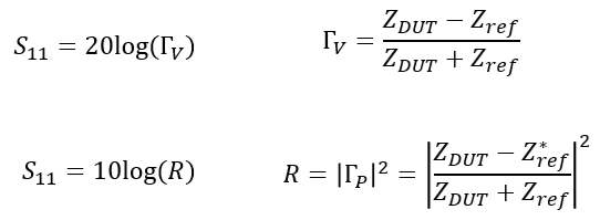
With these formulas, we can calculate an S11 value or return loss for a specific reflection value, or calculate the impedances for a specific amount of reflection or S11 value. Let's assume typical transmission lines for the moment, where the impedance is almost completely resistive.

10% power reflection: First, a −10 dB limit arises from exactly 10% power reflection. If we put 0.1 into the S11 formula based on the power reflection coefficient, we get:

S11 (R = 10%) = 10*log(0.1) = -10 dB

Now note that, because power is proportional to the square of voltage, a 10% power reflection corresponds to a 31.6% voltage reflection. However, if you put 31.6% reflection into the voltage reflection coefficient definition for S11, we still get a −10 dB value for S11:

S11 (Γ = 31.6%) = 20*log(0.316) = -10 dB

While this is certainly a less intuitive value for voltage amplitude reflection, it gives the same value for power amplitude reflection, as expected.

Now, what about a 10% voltage amplitude reflection? If we put this value into the voltage reflection S11 formula, we get the following:

S11 (Γ = 10%) = 20*log(0.1) = -20 dB

The −20 dB value is also to be expected due to the factor-of-two difference between the definitions for power and voltage.

S11 in Terms of Impedance Tolerance

If we were to take a 10% impedance tolerance and apply it in our reflection coefficient formula, we could then get an S11 value we would expect with this deviation from the target impedance value. Just for simplicity, let's take the standard 10% value that is normally specified on high-speed interfaces.

If we place the 10% tolerance value in the voltage reflection coefficient formula, we would have the following result for S11:

Γ = (0.1 / 2.1) = 4.76%

S11 (Γ = 4.76%) = 20*log(0.0476) = -26.44 dB

This is the same result you would get if you were to take the 10% impedance tolerance, calculate the power reflection coefficient, and calculate S11.

Just for fun, it is possible to calculate the impedance deviation that gives you a −10 dB value for S11, which I will leave as an exercise for readers. For a 50 Ohm reference impedance, it's easy to calculate that the transmission line impedance would need to be about 61 ohms, or just over 20% deviation!

What's the Significance of These Numbers?

10% impedance deviation and S11 = −10 dB are arbitrary in some ways, and they are not the only way we can qualify whether a channel will function as intended. This is especially true for digital designs, which require low return loss across a wide bandwidth in order to function correctly.

I think there is also some confusion with regard to the terminology. 10% impedance deviation is specified in terms of characteristic impedance, or the differential impedance if working with a differential pair, under the assumption that the transmission line has no losses or dispersion. However, the S11 value doesn't say anything about characteristic impedance; it is actually a measure of input impedance looking into a transmission line or circuit, and it is a measure across multiple frequencies.

Just as an example to see what we can infer from the graph, let’s look at a zoomed-in view of the graph shown above. At approximately 5.4 GHz, the SDD11 curve rises to -14.34 dB.

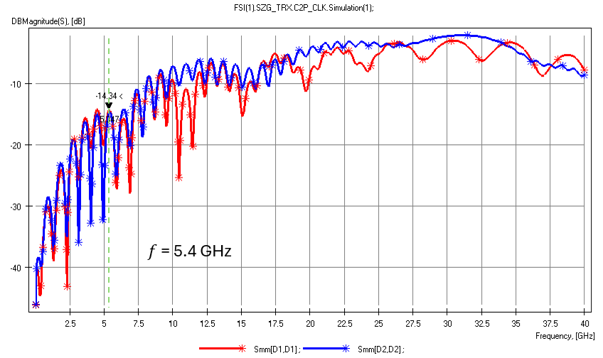
If we solve for the input impedance looking into the line in terms of the reflection coefficient, and use the definition of transmission line input impedance at maxima in the reflection spectrum, we find that the transmission line characteristic impedance can be calculated at each of these maxima as follows:

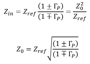
Note that we have included the aforementioned assumption that the line impedance is very nearly resistive.

With S11 = -14.34 dB, we find that the line’s differential impedance could be either approximately 122 Ohms or 82 Ohms; either value would produce the level of reflection seen above.

Ultimately, when the S11 curve rises above some critical value, the goal is to determine the line impedance and determine how it needs to be modified to satisfy channel/interface requirements. In addition, a low return loss value does not guarantee the interface will work. There are still timing constraints, crosstalk, ISI, and ultimately an eye diagram to examine to verify functionality of high-speed channels.

Whether you need to build reliable power electronics or advanced digital systems, use Altium’s complete set of PCB design features and world-class CAD tools. Altium provides the world’s premier electronic product development platform, complete with the industry’s best PCB design tools and cross-disciplinary collaboration features for advanced design teams. Contact an expert at Altium today!