Monte Carlo Simulation vs. Sensitivity Analysis: What’s the Difference?

In a previous article about circuit simulation and reliability, I looked at how Monte Carlo analysis is commonly used to evaluate circuits that are subject to random variations in component values. When we look specifically at components, there will always be some tolerances that will create variations in the electrical operating points of a circuit. These translate into some variation in the circuit’s output state, and the probable range of operating characteristics for your circuit.
Sensitivity analysis is a bit different and it tells you how the operating characteristics of your circuit change in a specific direction. Compared to a Monte Carlo simulation, sensitivity analysis gives you a convenient way to predict exactly how the operating characteristics will change if you were to deliberately increase or decrease the value of a component. It’s a very useful technique for justifying certain design decisions beyond looking at reliability from a statistical standpoint, and it gives you important insight into how your circuit responds to specific changes in component values.
Monte Carlo vs. Sensitivity Analysis
In Monte Carlo and sensitivity analysis, we are essentially doing the same thing: varying one or more components in a circuit, and measuring how the output responds. The difference is in how this is done: Monte Carlo applies random variations while sensitivity analysis applies a variation in a specific range chosen by the engineer.
Take component values as an example; in Monte Carlo, I know that component tolerances mean a component value would vary anywhere in the range of +/- (%tolerance), but I can’t predict what those specific values will be. In sensitivity analysis, I want to predict how the output changes if I deliberately change a component value by a certain amount, something which I get to choose as the engineer. The SPICE simulation engine in your design tools simply executes the standard circuit calculations using your random or selected component values.
The table below compares the nature of component value changes in Monte Carlo simulations vs. sensitivity analysis, as well as how the SPICE engine is used to generate results.
|
|
|
|
|
|
|
|
|
|
|
|
|
|
|
|
|
|
|
|
In the above table, I’ve mentioned component values as that is how Monte Carlo and sensitivity analysis are most often used. However, other factors like variations in a power supply level or variations in temperature can be examined with either type of simulation.
If I were to describe the operation of a circuit based on Monte Carlo analysis, my description would look like this:
- “The circuit is 95% likely to output between Voltage A and Voltage B; there is a 5% chance it is outside that range. The most likely operating point with X% probability is Voltage Y.”
Now, if I were to describe the operation of that same circuit based on sensitivity analysis results, my description would look like this:
- “If the value of Component X increases by Y%, the circuit output will change from Voltage A to Voltage B”
With this in mind, let’s look at an example of how to use sensitivity analysis results to better understand circuit behavior.
Example With a Voltage Regulator
For this example, we’ll return to our trusty voltage regulator circuit that I presented in the previous article about Monte Carlo simulations. Make sure to read that article if you want to see what your Monte Carlo results look like and how they are analyzed statistically. A schematic for this circuit is shown below.

In this example, we want to extract a specific linear model that defines how the output voltage varies with respect to changes in a specific component. Just for this example, we’ll look at variations in L1. Rather than vary L1 randomly, as we might do in a Monte Carlo simulation, We’ll vary it across a specific range so as to see how the output ripple changes for a given change in inductor L1. This would apply both in the continuous conduction mode and discontinuous/critical conduction mode.
Setup
In this example, suppose we want to see what happens to the ripple voltage if we change the value of L1 by +/-5% and +/-10%. To set these limits, you can open the Settings window from the Simulation Dashboard. Then open the Sensitivity Tab to configure the simulation.

In the above window, custom component limits for specific parts can be set to vary by a desired fraction during the simulation. For example, in the text boxes, simply enter 0.05 to shift the component value upwards by 5%. You could also set tolerance variations in the box in the top half of the window. Once these are set you can run one of the standard simulations, and the sensitivity analysis will run alongside the rest of your simulations.
Results
Transient analysis results up to about 0.3 ms are shown below. This window shows how the output voltage varies over time and how ripple varies with component values.

From this, we can see that increasing the inductance in L1 decreases the ripple. This is what we would expect based on the standard ripple formula for a buck converter. But can we go a bit further in quantifying this? Indeed we can by picking off the peak-to-peak ripple values, and then plotting these as a function of inductance. A graph for my data is shown below.

From the slope of the trendline, we can expect about 2.9 mV decrease in the peak-to-peak ripple per uH of inductance added to L1. This relationship holds out to +/- 10 uH. There is a bit of quantization error here from reading data off the graphs shown above, but the point of doing this analysis is clear: we can see exactly how our performance metric of interest changes with a simple numerical simulation.
Normally, we could calculate such a change for this particular circuit if we took the time to derive how the output LC filter (C2 and L2) transform the output from the regulator. It’s a bit of an involved calculation involving a derivative, but you could do the calculation by hand.
More Complex Circuits
What if the circuit was much more complex? Sensitivity analysis still applies even if you have a very complex circuit with multiple linear or nonlinear components. For example, suppose your circuit used multiple black box component models (such as our transistor model above), and it had many nonlinear components in complex arrangements (circuits with diodes, saturated transistors, etc.). In that case, sensitivity analysis in SPICE will give you the same answers very quickly precisely because it is a numerical simulation.
Summary and Comparison
To summarize, sensitivity analysis takes a similar approach to circuit analysis as Monte Carlo, but the interpretation of the results is very different. Monte Carlo tells you the statistically likely operating range of your circuit given known component tolerances. Sensitivity analysis tells you exactly how a system changes for a selected change in a component value.
If you’re analyzing circuit stability and reliability, both analyses are important. If you’re doing something like worst-case analysis (WCA), you’ll be using both methods together to analyze circuit behavior. I’ll look more at WCA in an upcoming article as it is very important in high-reliability electronics, such as in aerospace, automotive, medical, precision measurements and controls, and any other area where tolerances may create reliability challenges.
If you’re interested in running Monte Carlo simulations and sensitivity analysis for your circuits inside Altium Designer®, you’ll find these simulation tools built into the SPICE engine in the schematic editor. Once you’ve completed your PCB and you’re ready to share your designs with collaborators or your manufacturer, you can share your completed designs through the Altium 365™ platform. Everything you need to design and produce advanced electronics can be found in one software package.
We have only scratched the surface of what is possible to do with Altium Designer on Altium 365. Start your free trial of Altium Designer + Altium 365 today.

About Author
Related Resources


Related Technical Documentation

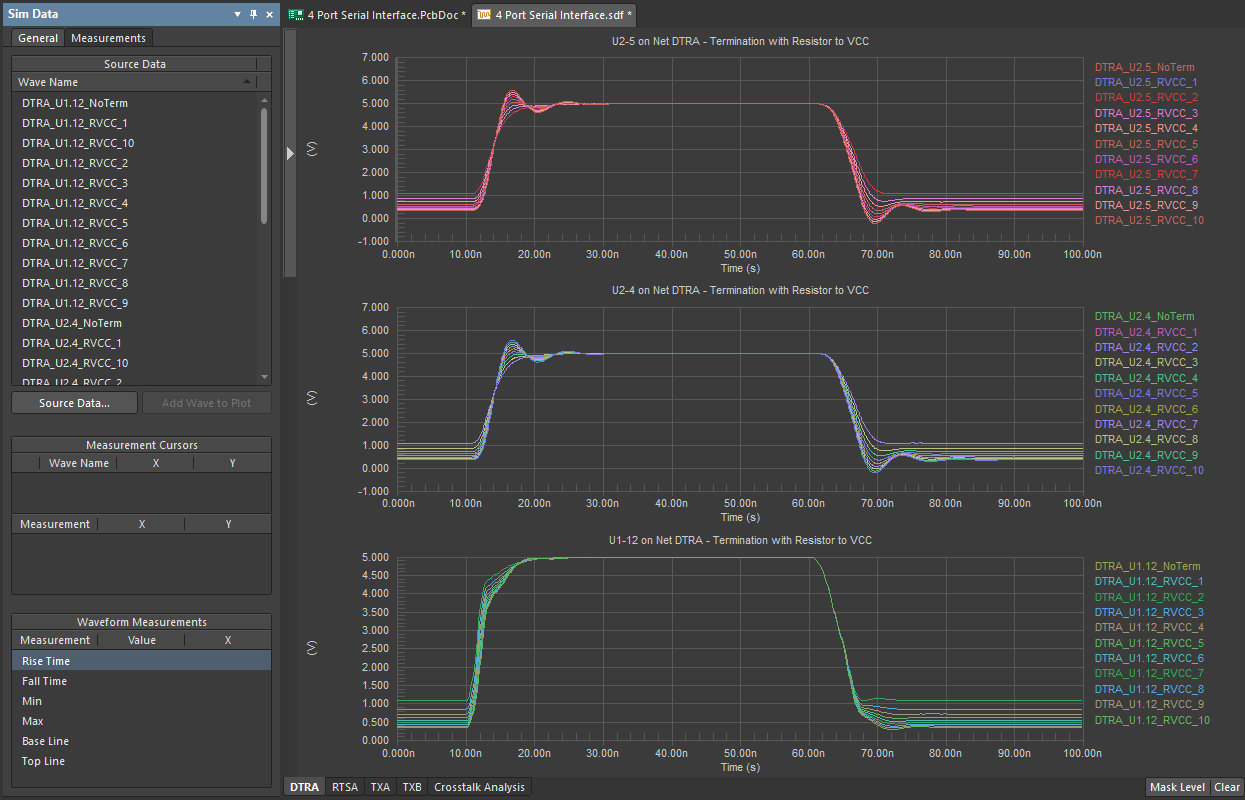


Table of Contents
Take advantage of the world's
most trusted PCB design system.
One interface. One data
model. Endless possibilities.
Effortlessly collaborate with
mechanical designers.
The world's most trusted
PCB design platform
Best in class interactive
routing
View License Options
Thank you, you are now subscribed to updates.