What is the Impedance of Length-Tuning Structures?

Recently, I received an excellent question from a YouTube viewer who was asking about differential pair routing and length tuning structures. This question (paraphrased) goes as follows:

Do length-tuning structures create an impedance discontinuity?

The answer is an unequivocal “yes”, but it might not matter in your design depending on several factors. The single-ended impedance of a trace in a differential pair will depend on the distance to the other trace, and applying a length-tuning structure is equivalent to changing the distance between the traces while meandering. Therefore, you will have a change in the odd-mode impedance of a single trace.

The question then becomes: does this deviation in trace impedance in a length tuning structure matter? Will it affect signal propagation behavior and signal integrity? It certainly will, and as a high-speed PCB designer, it’s your job to determine how much you should rely on length tuning to compensate for skew/jitter in your differential pairs.

Length-Tuning Structures Can Create Impedance Discontinuities

As we mentioned above, applying length-tuning structures to one side of a differential pair will create impedance discontinuities. These arise due to the following factors:

1. Single-ended (odd mode) and differential impedance are set by selecting a trace width AND trace spacing
2. Applying a length tuning structure creates a variation in trace spacing between the traces in the pair, therefore there will be a change in the impedance on one trace
3. This variation in impedance causes reflections from the input side of the differential pair
4. The signal speed on one end of the pair will be different in the length-tuning structure compared to the region with the traces running parallel

As a result of point #2 above, there will be some reflection experienced as a signal enters the length tuning section. The length tuning section can also create some mode conversion that is not accounted for in the process of delay tuning.

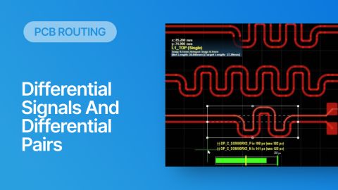
The image below summarizes the signal behavior observed in a differential pair due to the presence of a length-matching structure. The image below shows a situation where we are routing two different differential pairs on a laminate with Dk = 4.1 and substrate thickness 3.8 mil. The trace width, spacing, and impedances along each trace are shown along the length of the two routes.

Before the length-tuning section, the odd-mode impedance of the traces in each pair is 50 Ohms, so the differential impedance of each pair is 100 Ohms. Inside the length tuning section, we have something different. In the pair with larger spacing (10 mil), a 21 mil amplitude length tuning section has small sets of traces with odd-mode impedance of 53 Ohms. In the pair with smaller spacing (5 mil), the small traces in our 21 mil amplitude length tuning section have odd-mode impedance of 58.5 Ohms.

That’s a big difference! Decreasing the pair spacing by only 5 mils changes the impedance deviation from 6% to 17%.

The result is simple: for a length tuning section with a given amplitude (21 mil in this case), the impedance deviation due to length-tuning is smaller when the pairs started farther apart. This is another reason not to “tightly couple” differential pairs down to very small spacing; a little bit of spacing is actually beneficial to signal integrity!

Input Impedance Deviations Create Reflections

Inside the length tuning section, we see there is some impedance deviation, so there could be an input impedance mismatch. Just as is the case with any other impedance discontinuity along a transmission line, the discontinuity might not matter at low frequencies, but it will matter greatly at high frequencies.

How do you solve this problem? There are three possibilities:

1. Use wider spacing between the traces in the pair to minimize mismatch
2. Try to route so that you only need shorter length-tuning sections
3. Increase the trace width only in the loosely-coupled region

The first option is by far the easiest. The second option simply requires allowing for a slightly larger jitter at the receiver, which may not be possible without re-engineering the routing. The third option is not easily automated, but it is most effective at matching the length-tuning section’s input impedance to the parallel section’s impedance.

Propagation Delay Deviations Create Mode Conversion

In the above image, I showed the impedance but I didn’t show the propagation delay variation in each section. Because the impedance is different, the propagation delay will also be different. The image below summarizes the propagation delay in each region of the two length tuning sections shown above.

Here we see that the pair with wider spacing is also superior in terms of the deviation in the propagation delay. The 10 mil-spaced pair has a 2.4% increase in propagation delay, while the 5 mil-spaced pair has a 4.4% increase in propagation delay. Again, it’s a big difference and it should illustrate the superiority of slightly wider spacing between the two sides of the differential pair.

So who cares if the propagation delay is different by a few ps per inch in the length matching sections? The problem is in the vertical section, which will have a propagation delay that matches none of the values shown above. Once length tuning is applied, the result is mode conversion, or a conversion of common-mode noise into differential-mode noise. Take a look at the example for our coarsely-spaced pair shown below.

The reason this occurs is that length tuning tools are not using the modified propagation delay for time-based length-tuning. Instead, they are using the propagation delay value that assumes the two traces are routed in parallel. In the above example for the 10 mil-spaced pair, the routing tool uses 145.34 ps/in to apply the length tuning value, but the real propagation delay is somewhere between 145.34 ps/in and 148.89 ps/in.

In other words, the length tuning tool is assuming the signal travels faster along the length-tuning section than it will in reality. The result is some leftover mismatch in the phase response for each trace in the pair. The phase mismatch is also larger if you have a larger timing mismatch to compensate. The leftover phase persists even if the length tuning sections are the exact same length, so you then need to apply a longer length tuning section to eliminate the leftover phase mismatch, and the closer-spaced pair will require even more of this additional length tuning to compensate for phase! This leads to a vicious cycle of even more reflection.

We can see this if we calculate the phase response of each pair (phase of S21 and S43, or phase of the transfer function) from the transfer function of this differential pair. The graph below compares the phase of the transfer function for the 10 mil-spaced pair with length tuning included as shown above.

Why worry about this? The issue is not necessarily leftover skew; getting two traces in a differential pair to the exact same length will sufficiently align the signal swings on each side of the pair, which will minimize the total jitter. The problem with the phase response is that the total common-mode reduction capability of the receiver might be reduced, depending on the receiver’s bandwidth as defined by the Nyquist frequency. If the difference in the phase response is extreme and stretches below the Nyquist frequency, then the receiver will not be able to fully suppress common-mode noise. Expect about 10 dB reduction below the Nyquist frequency on longer length tuning sections.

Summary and Rules of Thumb

Because of the complexity of calculating the impedance deviation and high-frequency skew in a length-tuning structure, it’s difficult to account for it through an inductive calculation with the standard input impedance formula. 

Everything I’ve shown above should illustrate that tight coupling between differential pairs is a bit of a double-edged sword. From the discussion above, we can identify two appropriate rules of thumb for working with length-tuning structures:

1. If you need to apply length tuning, opt for slightly larger spacing between the pairs as this will reduce the impedance and propagation delay deviations.
2. When you do apply some length tuning, try to make it short to minimize reflections and mode conversion.

Point #2 is equivalent to the guideline “place direct routes between components”. Getting to a good rule of thumb is a bit difficult because that rule is going to relate 3 variables (rise time, spacing, and length tuning distance), but it’s something I’m interested in and will be writing more about in the future.

If you’ve already determined you need double termination (either DC or AC coupling), and you’ve already floor-planned well enough to ensure you’re routing straight into the receiver component, then you can use tighter coupling, just ensure the odd-mode impedance value of your traces will hit the termination value requried at the receiver's input. And of course, make sure you test your channel design, ideally with a test board on a similar stackup!

When you’re ready to route your differential pairs and quickly apply length tuning structures, use the best set of routing and layout features in Altium Designer®. You can also obtain highly accurate impedance calculations with an integrated field solver utility in the Layer Stack Manager utility as you create your PCB stackup. When you’re ready to share your designs with collaborators or your manufacturer, you can share your completed designs through the Altium 365™ platform. Everything you need to design and produce advanced electronics can be found in one software package.

We have only scratched the surface of what is possible to do with Altium Designer on Altium 365. Start your free trial of Altium Designer + Altium 365 today.