What is Propagation Delay in High Speed PCB Design?

Every electromagnetic signal, whether it's a digital signal traveling in a PCB or a wave propagating through the air between antennas, will have a finite speed. This finite speed is the propagation delay for a signal. It is an important quantity for several reasons, which are primarily found in high-speed PCB design and in RF systems design. Differential digital interfaces and phase-sensitive RF designs are the most important areas where propagation delay is important and becomes and important parameter in a PCB layout. 

In this article, I'll explain exactly where propagation delay is used in some basic calculations for PCB design. We'll see shortly that the important uses of propagation delay arise when we need to ensure consistent phase response across multiple interconnects in a PCB.

What is Propagation Delay?

Propagation delay refers to the inverse of the speed of a traveling electromagnetic signal. It is primarily used in the PCB industry to refer to signal speed, while integrated circuit designers use the same term to refer to the time required for a logic state to toggle from an input to an output. In a PCB, the propagation delay experienced by a signal is expressed in units of time per distance (inverse of speed). In other words, as long as you know the speed of light for a signal in a PCB, invert the value and you have the propagation delay.

When a PCB designer is planning a transmission line design for an impedance controlled interface, they may need to calculate the propagation delay for a signal on that line. The factors that determine the propagation delay of a signal include:

• Dielectric constant of the substrate
• The impedance value (really the geometry of the transmission line)
• The distance to the transmission line's reference plane(s)
• For a differential pair, the distance to the other trace in the pair
• Fiber weave effects in the PCB dielectric material

Definition for Striplines and Microstrips

The simplest definition comes from looking at the speed of light in vacuum; by using your PCB material's Dk value, you can determine the signal speed:

Invert this value, and you have the propagation delay in units of time per distance. A typical value for a 50 Ohm microstrip is ~150 ps/inch, and for striplines a typical value is ~171 ps/inch; both assume Dk = 4 dielectrics. Why should a microstrip have a different propagation delay compared to a stripline? This is because of the dependence of the geometry of the interconnect. For a stripline, the routing is on the surface layer and some of the electric field lines will pass through air, so the signal speed is defined using an "effective" Dk value:

Next, we need a formula for the effectivec Dk for microstrip lines. This value depends on the geometry of the transmission line and it can be calculated from Maxwell's equations. Using the quasi-TEM theory for transmission lines, it has been shown that the propagation delay for a signal on a microstrip is as follows:

Here, w and h are the width of the microstrip trace and the distance to the ground plane, respectively. This formula can be used by hand and is known to be accurate over a range of target impedance values within the quasi-TEM limit.

Definition From Transmission Line Theory

More generally, there is a definition for propagation delay that can be found directly from transmission line theory. This formula for the propagation delay requires you to know the distributed circuit element values for your particular transmission line:

Once again, invert this equation and you get the propagation delay.

This equation is universally true as a quasi-TEM model, but it is not so easy to use for design. Instead, it is normally used as part of a regression model, where the distributed element values in the formula are determined through an extraction process from network parameter measurements in an experiment or simulation. The processes and algorithms used for circuit model extraction are topics for another article.

Where Propagation Delay is Used

In general, you do not need to know or calculate the propagation delay for every single signal or trace connection on your PCB. 

Timing in High-Speed PCB Design

High-speed signals, whether they are on source-synchronous interfaces, on parallel buses, or on serial differential pairs, need to arrive at a receiver within some timing margin. In general, when the rise time of the signals are faster, the timing margin will be smaller. This means that the propagation constant must be known in order to apply length tuning, which ensures signals arrive within the required timing margin.

The main timing constraint that determines whether a high-speed interface will work is the timing mismatch between two signals, which we will call Δt. The relationship between the allowed length mismatch and the allowed timing mismatch is given by:

This length mismatch/timing mismatch arises in three important instances:

• Between signals in a parallel bus (such as DDR)
• Between two traces in a differential pair
• Between multiple differential pairs

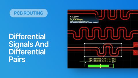
As an example of length tuning applied in a real situation, I like to show the below image of a CSI-2 interface on an FPGA with its escape routing. The image below shows five differential pairs (4 signal lanes and a clock lane) that make up a CSI-2 interface, which would normally be routed into a camera connector. We can see one length tuning section applied in the differential net AWR_3_CSI2_TX0, which ensures that the timing mismatch between these two traces is minimized. Because the design software knows the allowed timing mismatch (it's selected by the designer) and the propagation delay (it's set in the design rules), the PCB layout tool can check for a length mismatch by automatically applying the above formula.

The best PCB design software will automatically convert between the allowed timing mismatch and the actual length mismatch between two signals, but only as long as one of these constraints is defined in your design rules and the propagation delay is known. If your desingn software can perform an impedance calculation for your mismatched nets, then it can also determine the propagation delay for that specific transmission line geometry, and you won't have to calculate this by hand.

Determining Input Impedance

Another important area where a propagation delay calculation is needed, both in RF design and in digital design, is determination of input impedance. This is used to determine:

• Whether a signal will reflect at the input of an interconnect; it is used to determine an input reflection coefficient (S11 value);
• whether an impedance discontinuity is physically large enough to create noticable reflection in wideband (digital) signals.

In the former case, we want to determine whether an impedance matching network (stub or discretes) will produce the desired target input impedance. In the latter case, we want to determine at what frequencies a signal will begin strongly reflecting from an impedance discontinuity. The formula for determining the input impedance between a source and load connected with a transmission line is given in the image below:

From here you can do things like predict the exact frequencies at which a load and source will be perfectly impedance matched by a transmission line of length l and with characteristic impedance Z0.

Phase Response in RF Design

Finally, the other common instance where the propagation delay needs to be known is in the phase response of RF circuits. Some RF designs require engineering the phase response of a signal sourced into an interconnect. The phase response is also related to the propagation delay as follows:

In other words, when a signal with known frequency and propagation delay travels a distance L on an interconnect, we can calculate its phase shift. This phase response is used in areas like printed RF circuit design to account for any effects requiring interference, such as resonators and filters. For example, if you reuqire a phase measurement of an incoming signal with respect to some reference, you will need to know the phase shift of the signal along your interconnect, which requires knowing the propagation delay in the system.

The most important area where phase response matching applies in RF PCB design is in phased array antennas. These antennas are specifically used in high-resolution scanning radar, MIMO wireless systems, and unique mmWave sensors. These systems require phase matching across multiple antenna elements, and each antenna element will have a feedline connecting to a transceiver chip. Phase matching is required to direct beams to targets or mobile device users, and the correct way to enforce phase matching across the entire array is to implement length tuning, similar to what you would do in a large parallel bus of single-ended signals.

A simple example of a 4x series-fed patch antenna array (plus 2 dummy antennas) is shown below. Modern car radars have many more antennas, with virtual array sizes reaching hundreds of antennas.

In these systems, the operating frequency is typically in the mmWave range (at WiFi or above), so the transmission lines are typically routed as coplanar waveguides. The design equations for coplanar waveguides are quite different from standard microstrips, so an electromagnetic field solver may be required to determine the propagation delay for these lines.

Propagation Delay From Measurements or Simulation

It is possible to determine propagation delay from a measurement or simulation. There are two tools that determine the propagation delay:

• A return loss plot can be used to determine the round-trip propagation delay time.
• An insertion loss plot gives the one-way propagation delay, i.e., from port to port.

Measurement From Insertion Loss

Which one of these measurements should be used to determine propagation delay? The most accurate measure of propagation delay is the one-way propagation time for the interconnect, which is given by the insertion loss plot. More specifically, you need to look at the phase of the insertion loss plot to determine the propagation delay. The derivative of the phase as a function of frequency gives the propagation time between the input and output ports as follows:

The most accurate measurement is in a low-reflection channel, i.e., where we do not see any waves in the insertion loss plot and the phase of the plot adds up linearly. In reality, there is always some dispersion in the channel, so the propagation delay will be a function of frequency. Dispersion in PCB materials tends to cause a lower dielectric constant at higher frequency, so a measurement of propagation delay in the higher-frequency portion of the graph would result in a lower propagation time, i.e., faster signal speed.

We can see an example of such a measurement shown below, where the phase in the insertion loss plot is overlaid alongside the magnitude of the insertion loss. This example is for a single-ended via, but the same process would be used for a transmission line, a differential interconnect, a cable, or any other DUT which is a linear time-invariant (LTI) system.

If you know what to look for in this plot, you will see very clearly that this via is quite dispersive at high frequencies starting around ~30 GHz. This is not just due to the insertion loss, but also to the fact that the slope of the phase curve changes significantly above 30 GHz, while the slope looks relatively constant below 30 GHz.

If we export the phase data to Excel and calculate the derivative using finite differences, we can use the insertion loss propagation delay equation to see the dispersion. The plot below shows this calculation, and the result shows how the propagation delay varies significantly for waves traveling from port 1 to port 2.

The propagation delay plot shown above is typical for vias which are not fully impedance matched throughout the required impedance range. The range where the mismatch is largest (around 30 GHz) is showing the largest deviation in propagation delay from the low-frequency behavior.

So what is the big takeaway from this graph? It is that the via, which is not sufficiently impedance matched for high-bandwidth digital channels, will contribute to signal distortion at frequencies above ~20 GHz. The distortion becomes much larger above ~30 GHz, where the insertion loss plot rolls over and exhibits significantly more loss.

Measurement From Return Loss

What about a return loss plot? Can you or should you use a return loss plot to determine propagation delay? It is possible to do this, but it requires that the channel exhibit low reflection within the frequency band where the propagation delay is being calculated. If there is too much reflection or many discontinuities in the channel, the phase of the return loss curve can become very chaotic and exhibit many phase reversals. The result is that the propagation delay will be quite accurate.

Still, if you want to use the return loss plot to calculate propagation delay, you need to know that the phase is measured for the round-trip time, so the formula needed to calculate the propagation time would be:

Note that the factor of 2 appears in the denominator to account for the round-trip time in the channel.

If we take the corresponding return loss plot for the above insertion loss plot and plot S11 and S22, we can see something quite interesting: what appears to be different phase curves depending on which port (or in this case, which end of the via) is excited.

Given two different measures of propagation delay, I would trust the insertion loss measure more due to the reasons I cited above. Note, however, that both plots show that the channels are highly dispersive, but it is important to note the physical differences causing this: the transmitted signal (S21 plot) experiences loss-related dispersion (absorptive and radiated), while the reflected signal (S11 and S22 plot) shows how impedance discontinuities cascaded in different directions lead to dispersion in the reflected signal.

Whether you need to build reliable power electronics or advanced digital systems, use Altium’s complete set of PCB design features and world-class CAD tools. Altium provides the world’s premier electronic product development platform, complete with the industry’s best PCB design tools and cross-disciplinary collaboration features for advanced design teams. Contact an expert at Altium today!