Interplane Capacitance and PCB Stackups

This article is intended to provide insights on interplane capacitance and guidance for the process of designing PCB stackups. It is useful to look at the evolution of technology as time has passed in order to see how the demands on the PCB stackup have changed.

In the early days of PCB fabrication, logic circuits were so slow that the only concerns were how to make connections between logic or discrete parts and provide a path for the DC power to each part. All a needed to do was provide enough signal layers for all the wires, and enough copper in the power paths to deliver the DC power with a minimum of sag or droop. It did not matter what the glass cloth used in the laminate and prepreg was, or what the resin system was, or how thick each piece of laminate was. The goal was the lowest priced PCB that would stand up to the soldering process and be reliable.

Eventually ICs became fast enough that problems such as reflections and cross talk mattered. The logic family that did this was ECL. At that time, the primary users of ECL were large computer companies such as IBM, Control Data and Cray Research. These companies had engineers on staff who did the impedance calculations needed to design stackups, and had their own in-house PCB fabrication facilities as the public market fabricators did not yet have the capabilities to exercise control of fabrication necessary to meet their requirements.

In the mid-1980s TTL, the most common logic type then in use, became fast enough that reflections became a problem requiring PCBs to have controlled impedance. Few, if any, of the engineers designing with TTL and CMOS had any understanding of how to achieve a controlled impedance PCB, so they would demand that the fabricator deliver PCBs with a known impedance, usually 50 ohms. Fabricators did not have this capability as their skill set included plating, etching lamination and drilling. Still, engineers demanded that the fabricators do the impedance calculations. The author was around during this time and spent many hours helping fabricators develop the ability to calculate impedance. Their skill at this task was very hit and miss and, in many cases, still is today.

Soon after this, crosstalk between traces running side by side became an issue requiring designers to take care on how close, side-to-side and over and under traces were routed.

By the mid-1990s, speeds had increased to such an extent that most products were failing EMI due to the need for capacitance that worked above 100 Mhz. None of the discrete capacitors placed on the power rails could solve this problem due to their mounting inductance. This gave rise to what is known as interplane capacitance or buried capacitance. Interplane capacitance is created by placing the power and ground planes very close to each other, typically, less than 3 mils.

So, now we have three demands placed on stackup design: controlled impedance, crosstalk control, and the need for interplane capacitance. Some fabricators could get the impedance right in a stackup, but there is no way for them to account for the other two. This responsibility rests with the design engineer who is the only one who knows what is needed and how to implement the required control.

By the mid-2000s, speeds of many differential pairs got so fast that the glass weave used in the laminate and prepreg could induce a phenomenon known as skew that destroyed the signal. Skew is the misalignment of the two sides of a differential pair as they arrive at the receiver. In addition, losses in the laminate began to affect these high-speed signals, forcing the engineering team to seek low loss laminates that satisfied loss goals as well as all the above requirements. A detailed discussion of materials available to satisfy all these needs is contained in Chapter 3 of this document.

For all the reasons discussed above, the design engineer must take charge of design. To do this successfully a thorough understanding of the fabrication process and materials is essential. This section will cover all the topics involved in designing of PCB stackups that meet the four constraints: controlled impedance, managing crosstalk, creating adequate interplane capacitance, and specifying the correct weave to manage skew.

Arranging Layers With Interplane Capacitance in Mind

Once the number of power planes, ground planes, and signal layers have been determined for a given design, arranging them in such a way that all signal integrity rules are complied with and power delivery needs are met is a series of tradeoffs. If there is a need for interplane capacitance it will be necessary to arrange the layers so that ground and voltage planes are spaced close to each other. Figure 2.1 is an example of making tradeoffs between routing layers and power plane capacitance for a ten-layer PCB. The stackup on the left side of Figure 2.1 has six signal layers, but only has one pair of planes closely spaced. This is good for routing space, but not so good for power delivery if there is a need for interplane capacitance. The stackup on the right has only four routing layers (the two outer layers are too far from the nearest plane to achieve the proper impedance), but it now has two sets of plane pairs. This is good for interplane capacitance, but not as good for routing space.

Figure 2.1 Two Possible Ways to Arrange the Layers in a Ten Layer PCB.

In both cases above, all the signal layers are mated with planes across pieces of laminate except the two outer layers. As mentioned earlier, these layers will be too far from the nearest plane to achieve the proper impedance. They can be used for power traces and component mounting pads.

Once the arrangement of layers has been determined, the next step is to select the thickness of each dielectric layer to achieve the best performance at the lowest cost. To minimize crosstalk, it is advisable to select the thinnest laminate that meets SI goals for the space between signal layers and their plane partners. Once this is done, the trace width needed to achieve the target impedance is calculated. Following this, the thickness of the prepreg between the power planes is selected to satisfy the breakdown voltage requirements, and allow enough resin to fill the voids in the adjacent planes. This will usually be a single glass ply that begins three mils thick and presses down to about 2.5 mils.

In the example on the right in Figure 2.1, there are three prepreg layers that remain to be chosen. These are the one in the center of the stackup and the two just below the outer layers. (The outer layers in this stackup are not usable as controlled impedance layers, so their height above their underlying planes is not critical.) The thickness of all three of these spaces can be used to add material in order to arrive at the final thickness desired as changes in thickness in these three areas have little effect on the overall performance of the PCB.

Interplane Capacitance and the PDN Impedance

In modern designs, SI and PI engineers refer to the PDN impedance, rather than looking only at pulse travel times the way we did in earlier days with slower logic. PDN impedance is related to the amplitude of a transient response observed on the power rail. The goal is to keep the PDN impedance as low as possible so that current pulses into the digital IC do not create strong voltage transients on the power rail, which would create noise observed at all branches in the PDN.

The PDN impedance is related to the interplane capacitance, as well as the capacitance of all other capacitors in the PDN. However, all of these elements also have inductance. This is why the PDN impedance image shown below shows dips and peaks; the dips are associated with capacitor self-resonances, while the upward-sloping portions of the curves are associated with the inductance of capacitor packages/mounting features in the PCB.

PDN impedance plot showing dips at capacitor self-resonances and upward-sloping inductive regions. Learn more in this article.

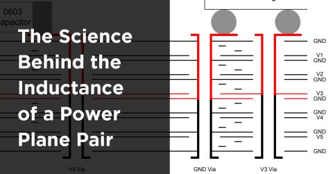
Spreading Inductance of the Plane Pair

The plane pair in a PCB stackup is not a pure capacitor. Current flowing from a decoupling capacitor network, across the power plane, into the load IC, and returning along the ground plane creates a current loop that has its own inductance contribution. This inductance contributed specifically by the planes is called the spreading inductance. The term reflects the fact that current does not follow a straight line between the capacitor via and the IC power pin; instead, it spreads outward in the copper, occupying a region that is wider than the via-to-via spacing but that does not fill the entire plane area.

Spreading inductance is expressed as a per-square value, typically on the order of picohenrys per square. For common PCB stackup geometries, the spreading inductance of a tightly spaced plane pair falls in the range of tens of picohenrys. Two geometric parameters control this value: the lateral distance between the decoupling capacitor and the load IC, and the dielectric thickness separating the power and ground planes. Reducing either distance reduces the spreading inductance. Increasing the overall plane area beyond a certain point does not help, because the current has already stopped spreading before it reaches the plane boundary.

The loop area between the power and ground plane defines the spreading inductance of the plane pair. Learn more in this article.

This inductance sets a practical ceiling on the frequency range over which the plane pair can effectively supply decoupling. Combined with the plane capacitance, the spreading inductance creates a self-resonance in the plane pair, typically somewhere in the range of 100 MHz to 1 GHz depending on geometry. Above that resonance, the plane pair impedance becomes inductive and rises with frequency, meaning the planes alone can no longer maintain low PDN impedance. Addressing PDN impedance above this range requires on-die and on-package capacitance, or the use of specialty stackup materials that push the plane-pair resonance higher.

Embedded Capacitance and Interplane Capacitance

Standard FR4 laminates separating a power and ground plane provide some interplane capacitance, but the amount is limited by the dielectric constant and the minimum practical laminate thickness (typically 2 mil or greater with standard glass weaves). When this capacitance is insufficient to meet PDN impedance targets in the 100s of MHz range, embedded capacitance materials offer a direct path to higher plane capacitance without adding discrete components. These materials are copper-clad laminates engineered with very thin dielectric layers (as low as 0.3 mil) and elevated dielectric constants (ranging from 3.5 up to 30, depending on the product). Placing an ECM between a dedicated power layer and a ground plane in the stackup increases the capacitance density of that plane pair by roughly an order of magnitude or more compared to a standard FR4 core of typical thickness.

Embedded capacitance material in a PCB stackup.

The effect on PDN impedance is twofold. First, the higher capacitance lowers the baseline impedance of the plane pair across a broad frequency range. Second, the moderately high loss tangent of most ECM formulations damps the resonant peaks that appear near 1 GHz in the plane pair response, reducing the Q-factor of those resonances. The result is a flatter, lower-impedance PDN profile through the frequency range where IC packages demand fast transient current. Measured data from DuPont and others confirm that thinner ECMs produce visibly lower PDN impedance and smaller resonant peaks near 1 GHz, which translates directly into reduced power bus ripple, less jitter in eye diagrams, and lower radiated EMI from board edges.

The reason planes and ECMs are so effective in this frequency range comes down to inductance (specifically, spreading inductance of the plane pair). AMD's Ultrascale PCB design guidance, for example, cites plane inductance values of 32 pH/square/mil (the distance unit accounts for the dilectric thickness). Compare this to the total loop inductance of a discrete decoupling capacitor, which includes the component ESL plus the via and pad mounting inductance and typically sums to roughly 1 nH or more. The plane pair's inductance is therefore one to two orders of magnitude lower than the inductance associated with a discrete capacitor's mounting structure. This is precisely why interplane capacitance, whether from standard laminates or ECMs, is the only practical decoupling mechanism that can maintain low PDN impedance out to approximately 1 GHz. Discrete capacitors simply cannot respond fast enough to provide stable power into the GHz range because of their ESL values and mounting inductance.

PCB Stackup Documentation

As the speeds of signals continue to increase, the demands placed on the PCB become more complex. Some of those demands, as mentioned above are controlled impedance, controlled crosstalk, interplane capacitance, managing path loss, and glass weave style control.

For these reasons, the documentation required has become more complex as well. The stackup drawing must contain more information than in the past, and the fabrication notes will need to be expanded. Figure 2.2 is an example of the amount of information that must be included in the stackup drawing to ensure the PCB is correctly fabricated. Notice that there is no impedance information on the stackup drawing. The reason for this is that all the other requirements must also be met. Therefore, the stackup drawing specifies the overall cross-section of the PCB that meets all the SI goals. The design engineer must determine all of these including impedance and specify the total cross section.

Figure 2.2 A Stackup Drawing with Adequate Information

For signal integrity reasons, the design engineer must take charge of the overall stackup design including determining the trace widths necessary to achieve the impedance goals. However, the guidance of the engineers at the fabricator is required to insure the stackup has been optimized for manufacturability.

Interplane Capacitance and Other Calculations Required When Designing a Stackup

As mentioned earlier, there are a number of calculations that must be made to arrive at a final stackup drawing and the routing rules for a design. Among these are:

• Impedance

• Cross talk spacing

• Interplane Capacitance required

• Allowable trace loss

• Allowable skew

Impedance Calculation

The most accurate method for calculating impedance is with a tool that uses Maxwell’s equations. The least reliable method is to use any of the equations that were once the only choice. There are a number of products on the market that use Maxwell’s equations in a 2D field solver. Any of these produce accurate answers provided the correct dielectric constants are used. The correct dielectric constant for each type of laminate is obtained from the laminate manufacturer’s laminate information. Table 2.1 is a typical laminate information sheet with dielectric constant (er or Dk) as a function of frequency. Notice that the Dk varies with both resin content and frequency. It is imperative that the correct value is used when calculating impedance. Unfortunately, the author has discovered that many fabricators do not use the correct Dk values when calculating impedance, resulting in PCBs that are fabricated with the wrong impedance.

Information courtesy of Isola

Table 2.1 A Typical Laminate Information Table

Accurate impedance prediction in a PCB stackup requires a field solver that accounts for trace geometry, dielectric properties, copper roughness, and layer-to-layer coupling. Several commercial tools are available for this purpose:

• Polar Instruments Si8000 and Si9000 are widely used by fabricators and designers for controlled-impedance stackup calculations and coupon modeling.
• Simbeor from Simberian provides electromagnetic extraction with high accuracy for both single-ended and differential transmission line structures.
• Ansys HFSS and Q3D Extractor offer full-wave and quasi-static extraction for complex geometries where 2D approximations are insufficient.

The Layer Stack Manager in Altium Designer integrates impedance calculation models derived from Simbeor's electromagnetic solver technology. These models provide accurate characteristic impedance predictions for single-ended and differential trace geometries directly within the stackup editor, without requiring a separate tool or export step. The Simbeor-based models are well validated against measurements and full-wave solvers, and they account for the trace cross-section, dielectric layer geometry, and reference plane configuration in the stackup. For designers working through stackup iterations, having this level of accuracy embedded in the design tool eliminates a significant back-and-forth step with external calculators.

The impedance values produced by these models are lossless characteristic impedance values, meaning they do not account for conductor loss, dielectric loss, or copper roughness effects that would modify the impedance at high frequencies. In practice, the lossless value serves as a very good starting point for predicting the lossy impedance that a fabricated board will exhibit, because the real part of the characteristic impedance converges toward the lossless value at frequencies above a few hundred MHz for most PCB geometries. Designers can use the lossless result from the Layer Stack Manager to set their target impedance and then apply loss corrections in a downstream simulation if needed.

This feature is included as a standard feature in Altium Designer. To perform the impedance calculations in this tool, follow these steps:

• Open your PCB in the PCB editor.
• Go to Design -> Layer Stack Manager.
• In the Layer Stack Manager document, click the Impedance tab (at the bottom).
• Click Add Impedance Profile (or the + button) to create a profile and use the Properties panel to set Type, Target Impedance, and other parameters (the tool will calculate width/gap based on your inputs).

To learn more, read the Altium Documentation.

Crosstalk Spacing Calculation

Crosstalk is the unwanted interaction between two traces that are spaced too close together. The stackups in Figure 2.1 have pairs of signal layers one over the top of the other. If a signal in one of those layers lies over the top of one in the other layer, the crosstalk will grow so rapidly that no amount of overlay at the speeds of current technology can be permitted without causing a crosstalk problem. The only safe routing strategy in this case, is to route one layer in the X direction and the other in the Y direction.

When traces run side-by-side in the same layer, care must be taken to make sure the spacing between traces and the height of the nearest plane is such that crosstalk goals are met. The only way to arrive at reliable spacing rules is to employ one of the simulation tools meant for the purpose. Rules such as 2H or 3H are arbitrary and unsafe to use.

Interplane Capacitance Calculation

Interplane capacitance, the capacitance formed by two planes closely spaced to each other, has proved necessary to provide the very rapid switching currents needed by modern logic to drive transmission lines and supply current to IC cores. Failure to include enough interplane capacitance in a design is the most common source of EMI failures.

Determining the amount of interplane capacitance needed is accomplished by employing one of the analytical tools designed for this purpose. The PCB stackup design cannot be completed without performing this analysis.

Determining the amount of interplane capacitance required for proper power delivery system operation must be completed before the stackup design can be done.

Allowable Trace Loss

As the speeds of data links continue to rise, the potential for signal degradation due to losses along the length of the signal paths, from losses in the dielectrics and copper can become significant. Deciding whether the loss in a proposed path is acceptable based on trace width and the loss properties of the dielectric is a complex analysis that requires a tool such as ADS, HFSS, Hyperlynx Gigahertz or similar tool.

There are a number of laminates on the market that have been engineered for very low loss. Deciding when a design needs one of these depends on four things. These are:

• Length of the signal path

• Frequency content of this signal

• Ability of the transmitter/receiver pair to compensate for loss

• Roughness of the copper in the planes and on the traces

Trace width is not on this list because it has been shown that for the allowable trace widths in most designs, changing trace width to reduce loss (making traces wider), is not a useful method for reducing loss.

Allowable Skew

Skew is the misalignment in time of the two signals in a differential pair as they arrive at the receiver. The primary source of unwanted skew is differences in travel time on each trace due to the uneven way in which the fibers in the glass weave are spaced. As the speeds of differential pair links continue to increase, the effect of an incorrect weave can cause a design to fail due to excess skew. 

Design the Stackup with Confidence

Modern PCB stackups demand more than rules of thumb and fabricator estimates. With Altium Develop, engineers take full control of impedance, losses, crosstalk, skew, and interplane capacitance directly in the design flow. The built‑in Stackup Manager, powered by Simbeor field‑solver technology, gives you Altium‑grade accuracy without heavyweight processes, so small and focused teams can design with confidence from first pass to release.

Get started with Altium Develop and move faster from design to manufacturable reality without unnecessary friction →