How to do PCB Trace Length Matching vs. Frequency

If you read many PCB design guidelines, particularly on parallel protocols and differential pair routing, you’ll see many mentions of trace length matching. When you need to do trace length matching in PCB design, your goal is to minimize timing differences between traces in a length-matching differential pair in a serial protocol, multiple traces in a parallel protocol (e.g., DDR data lines), multiple traces/pairs in a parallel protocol, or any protocol that uses source-synchronous clocking. CAD tools make it easy to consider what happens exactly at a single matching frequency. However, what happens at other frequencies? More specifically, what happens with broadband signals? In this blog, we're going to tackle length-matching guidelines.

All digital signals are broadband signals with frequency content extending from DC to infinity. Because of the broad bandwidth of digital signals, which frequency should be used for trace length matching? Unfortunately, the frequency used for trace length matching is ambiguous, so designers need to understand how to confront PCB trace length matching vs. frequency. To better understand this, we need to look at techniques used in broadband design and how to consider the entire signal bandwidth in trace length matching.

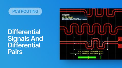
PCB Trace Length Matching vs. Frequency for Differential Pairs

Performing PCB trace length matching vs frequency correctly requires considering the entire bandwidth of a propagating signal on a trace. This has been a research topic for differential serial protocols over the last several years, and standards like USB 4 place specific requirements on broadband signal integrity metrics. Some example broadband signal integrity metrics are:

• Integrated differential crosstalk
• Integrated differential insertion loss
• Integrated differential return loss
• Integrated differential impedance deviations

By “integrated,” we mean that the particular aspect of signal integrity applies throughout the relevant matching frequency range. In other words, if we take differential crosstalk as an example, we want to minimize differential crosstalk between two differential pairs below some limit, which is specified in signaling standards. We’ll see why this is important for trace length matching in PCB design in just a moment.

Dispersion

In the time domain, we only care that the two ends of the differential pair cross the halfway transition between the HI and LOW states (assuming binary) at the same instant in time. Obviously, jitter creates a problem here in that it limits your trace length matching in PCB designs to some minimum tolerance, so you will never have two ends of a pair perfectly transition at the same instant. In the frequency domain, we need to account for dispersion from the following sources:

• Geometric dispersion: This arises due to the boundary conditions and geometry of an interconnect, which then determines the impedance of the interconnect as a function of geometry.
• Dielectric dispersion: This occurs in the PCB substrate and exists regardless of the geometry of an interconnect on the PCB. It includes both dispersion in Dk and loss.
• Roughness dispersion: This additional source of dispersion arises due to the causality of copper roughness models and the skin effect at high frequencies.
• Fiber weave dispersion: The fiber weave in a PCB laminate creates periodic variations in dispersion throughout an interconnect.

Because these sources of dispersion always exist for traces, they cause impedance, velocity, and all other signal integrity metrics for a real PCB trace to be functions of frequency. An example showing how dispersion in the real part of Dk can affect the impedance of a microstrip trace is shown below.

Signal Velocity

If you’re familiar with transmission line theory, you know that impedance and signal velocity are intimately related. Let’s look at the signal velocity on a PCB trace as an example; the graph below shows the group velocity and phase velocity for a simulated stripline with roughness and dispersion.

Here we can see that the phase velocity varies significantly over a very broad range of frequencies, reaching a factor 2 variation from 1 MHz up to 20 GHz. The variation in the phase velocity is the important parameter here as this is the rate at which different frequency components travel along an interconnect. With this variation, we can see how PCB trace length matching vs. frequency becomes difficult for real interconnects; we need some way to take account of all frequencies, not just a single frequency chosen arbitrarily.

Broadband PCB Length Matching vs. Frequency

We should consider the minimum allowed length deviation for a given signaling standard to formulate a metric for length matching in PCB design. Let’s call this minimum time deviation tlim. We can write the following equation relating the length tolerance and allowed timing mismatch:

Here, the function k is just the propagation constant for signals on the interconnect, and this is also a function of frequency due to dispersion. We can take a statistical approach to deal with the allowed length mismatch using something called an “Lp norm”. Without going too deep into the math involved, just know that this metric is equivalent to calculating the RMS variation between a function and some mean value (they only differ by a constant). Therefore, this makes it an ideal mathematical tool for accounting for variations between some target design value and a signal integrity metric (impedance, impulse response decay/delay, crosstalk strength, etc.).

Using the Lp norm, we can rewrite the allowed length mismatch in terms of some upper limit defined from the timing mismatch limit tlim:

When working with broadband signal integrity metrics for PCB design, the above equation can be viewed as a constraint: as you size the transmission line, this can affect the total allowed length deviation between two ends of a differential pair, or between any two traces in a high-speed parallel protocol. The integral is rather easy to calculate as long as you know the propagation constant for the transmission line. This can then be calculated using a field solver, or by hand using an analytical model with a standard transmission line geometry as I’ve discussed in an earlier article.

Just to give some numbers for this calculation, if I take the phase velocity for the simulated stripline I’ve shown above, we find that the maximum allowed length mismatch between two single-ended fully isolated traces in parallel is 2.07 mm if the maximum allowed timing mismatch is 10 ps. Note that, for 10 ps, this is a significant fraction of the edge rate for many high-speed digital signals. For example, in OpenVPX backplanes my firm designs, we set the edge rate limit to 6 ps for 10G Ethernet signals. For the stripline I’ve simulated above, this would equate to 1.3041 mm of allowed length mismatch.

In summary, we’ve shown that PCB trace length matching vs. frequency can be reduced to a single metric using an Lp norm. If you’re a PCB designer, you don’t need to perform this calculation manually, and you just need to use the right set of PCB routing tools. The routing engine in Altium Designer® includes an integrated electromagnetic field solver from Simberian, which accounts for broadband impedance and signal speed variations in your PCB substrate. Learn more about length matching for high-speed signaling standards in this tutorial.

When you’ve finished your design and want to share your project, the Altium 365™ platform makes it easy to collaborate with other designers. We have only scratched the surface of what is possible to do with Altium Designer on Altium 365. You can check the product page for a more in-depth feature description or one of the On-Demand Webinars for more information on PCB length matching in differential pairs.